Ch. 9 – Synchronization

Load libraries

#if (!require(devtools)) install.packages("devtools",quiet=TRUE)
#devtools::install_github("tuomaseerola/onsetsync")
library(onsetsync)
library(dplyr,quiet=TRUE)
#install.packages("cowplot",quiet=TRUE)
library(cowplot)

Explore synchronisation in Cuban Salsa and Son

Take an example track from IEMP corpus and visualise beats and calculate the synchronies.

set.seed(1234)
CSS_Song2 <- onsetsync::CSS_IEMP[[2]]
fig1 <- plot_by_beat(df = CSS_Song2, 
                     instr = c('Bass','Clave','Guitar','Tres'), 
                     beat = 'SD', 
                     virtual = 'Isochronous.SD.Time',
                     pcols = 2)
inst <- c('Clave','Bass','Guitar','Tres') # Define instruments 
dn <- sync_execute_pairs(CSS_Song2,inst,100,1,'SD')
fig2 <- plot_by_pair(dn)  # plot
G <- cowplot::plot_grid(fig1,fig2,nrow = 2)
print(G)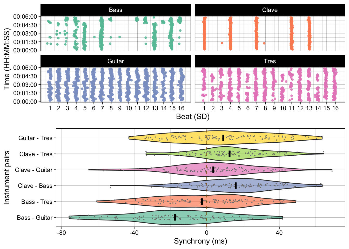

round(mean(dn$asynch$`Clave - Guitar`)*1000,1)

[1] 3.6

round(mean(dn$asynch$`Clave - Bass`)*1000,1)

[1] 15.9

round(mean(dn$asynch$`Bass - Guitar`)*1000,1)

[1] -17.6

round(mean(dn$asynch$`Bass - Tres`)*1000,1)

[1] -2.7

References

Poole, A. (2021). Groove in Cuban Son and Salsa Performance. Journal of the Royal Musical Association, 146(1), 117-145. doi:10.1017/rma.2021.2