import numpy as np
import pandas as pd
import librosa
import librosa.display
import IPython.display as ipd
from matplotlib import pyplot as plt
from tqdm.auto import tqdm
%matplotlib inlineCh. 11 – Genre classification
Figure 11.2. Illustration of genre classification with acoustic descriptors. Panel A and B: Distribution of RMSE and Spectral centroid values across 10 genres in all excerpts. Panel C: Confusion matrix of the random forest classification model showing the proportion of cases predicted in the actual and predicted genres.
Summary
This notebook will look at a classic genre categorization study and dataset by Tzanetakis & Cook (2002) and will conduct a simple classification of genre based on acoustic features extracted from the audio files. The full data contains 100 audio excerpts from 10 different genres (1000 clips in total), but we are going to start with a smaller set to keep this light to run. It should be noted that the selection of the excerpts for this dataset were not particularly rigorous and represented the collection of music that George Tzanetakis had at his disposal at the time. And this dataset has some quirks and imperfections, but I think it is still a fun, classic and illustrative example to explore.
Setup
Load libraries
Load dataset
We first install mirdata library to the computer.
import sys
!{sys.executable} -m pip install mirdata
Then we initialise the library and download the audio excerpts needed. I only take 100 excerpts here but you can take all 1000 excerpts by altering the script below.
import mirdata
#print(mirdata.list_datasets())
gtzan_genre = mirdata.initialize('gtzan_genre')
gtzan = mirdata.initialize('gtzan_genre', version='mini')   # This is 100 excerpts
#gtzan = mirdata.initialize('gtzan_genre')                  # This is 1000 excerpts (uncomment if you want to analyse the full data)
gtzan.download()
print('Downloaded',len(gtzan.track_ids),'tracks')
INFO: Downloading ['mini', 'tempo_beat_annotations'] to /Users/tuomaseerola/mir_datasets/gtzan_genre
INFO: [mini] downloading main.zip
INFO: /Users/tuomaseerola/mir_datasets/gtzan_genre/main.zip already exists and will not be downloaded. Rerun with force_overwrite=True to delete this file and force the download.
INFO: [tempo_beat_annotations] downloading annot.zip
INFO: /Users/tuomaseerola/mir_datasets/gtzan_genre/annot.zip already exists and will not be downloaded. Rerun with force_overwrite=True to delete this file and force the download.Downloaded 100 tracksLet’s look at an example (track ID 88).
ID = 88
tracks = gtzan.load_tracks()
ex = tracks[gtzan.track_ids[ID]]
print(["Genre:", ex.genre, "Name:", ex.track_id, "Tempo:",ex.tempo,])
print(ex.audio[1])
plt.figure(figsize=(8, 2))
librosa.display.waveshow(y = ex.audio[0], sr = ex.audio[1])
ipd.display(ipd.Audio(data = ex.audio[0], rate = ex.audio[1]))
['Genre:', 'pop', 'Name:', 'pop.00008', 'Tempo:', 84.1]
22050
Extract features
Let’s extract some features and use them to predict genres. We take some rhythm features, some timbral features, _MFCC_s (19 in total), and chromas (12 in total). In the feature extraction, we calculate the features across the 30-second excerpt and then just take the mean to represent the feature.
The summary of the track could be more sophisticated (one could take the median, and the standard deviation, for instance, or to avoid extreme values, or to take multiple measures from within each example, and using bagging or voting where separate clips are used in assessing the most likely genre. This latter goes close to ensemble machine-learning techniques).
df = pd.DataFrame(columns = ['genre','bpm','rmse', 'spec_cent','spec_bw','rolloff','zcr','spec_ctr','mfcc1','mfcc2','mfcc3','mfcc4','mfcc5','mfcc6','mfcc7','mfcc8','mfcc9','mfcc10','mfcc11','mfcc12','mfcc13','mfcc14','mfcc15','mfcc16','mfcc17','mfcc18','mfcc19','chroma1','chroma2','chroma3','chroma4','chroma5','chroma6','chroma7','chroma8','chroma9','chroma10','chroma11','chroma12'])
for track in tqdm(tracks):
  ex = tracks[track]
  y, sr = librosa.load(ex.audio_path)
  chroma_stft = librosa.feature.chroma_stft(y=y, sr=sr)
  rmse = librosa.feature.rms(y=y)
  spec_cent = librosa.feature.spectral_centroid(y=y, sr=sr)
  spec_bw = librosa.feature.spectral_bandwidth(y=y, sr=sr)
  rolloff = librosa.feature.spectral_rolloff(y=y, sr=sr)
  zcr = librosa.feature.zero_crossing_rate(y)
  spec_ctr = librosa.feature.spectral_contrast(y=y, sr=sr, hop_length=512)
  chroma = librosa.feature.chroma_stft(y=y, sr=sr, hop_length=512)
  mfcc = librosa.feature.mfcc(y=y, sr=sr)
  df.loc[len(df)] = [ex.genre,ex.tempo,np.mean(rmse),np.mean(spec_cent),np.mean(spec_bw),np.mean(rolloff),np.mean(zcr),np.mean(spec_ctr),np.mean(mfcc[1]),np.mean(mfcc[2]),np.mean(mfcc[3]),np.mean(mfcc[4]),np.mean(mfcc[5]),np.mean(mfcc[6]),np.mean(mfcc[7]),np.mean(mfcc[8]),np.mean(mfcc[9]),np.mean(mfcc[10]),np.mean(mfcc[11]),np.mean(mfcc[12]),np.mean(mfcc[13]),np.mean(mfcc[14]),np.mean(mfcc[15]),np.mean(mfcc[16]),np.mean(mfcc[17]),np.mean(mfcc[18]),np.mean(mfcc[19]),np.mean(chroma[0]),np.mean(chroma[1]),np.mean(chroma[2]),np.mean(chroma[3]),np.mean(chroma[4]),np.mean(chroma[5]),np.mean(chroma[6]),np.mean(chroma[7]),np.mean(chroma[8]),np.mean(chroma[9]),np.mean(chroma[10]),np.mean(chroma[11])]
Explore features
Let’s look at some of features across genres. Are there differences in dynamics or brightness?
       rmse    spec_cent      spec_bw      rolloff       zcr   spec_ctr
0  0.036233  1505.357461  1559.228895  2717.238764  0.098223  23.372866
1  0.030610  1361.006486  1441.739951  2389.011463  0.087766  25.186866
2  0.043828  1490.274810  1600.005082  2785.418914  0.090046  22.894315
3  0.029426  1526.628932  1499.462050  2916.150271  0.108946  25.663545
Feature space
How large is our feature space and do have features that are redundant, that is highly similar to each other? This can be easily explored by visualising the correlations between all features.
corr = df.iloc[0:99,1:27].corr() # Compute the correlation matrix
mask = np.triu(np.ones_like(corr, dtype=bool))       # Generate a mask for the upper triangle
f, ax = plt.subplots(figsize=(8, 8))                # Define matplotlib figure
cmap = sns.diverging_palette(230, 20, as_cmap=True)  # Custom colormap
sns.heatmap(corr, mask=mask, cmap=cmap, vmax=1.00, center=0,
            square=True, linewidths=.5, cbar_kws={"shrink": .5}) # Draw the heatmap with the mask and correct aspect ratio
plt.show()
Classification and machine-learning algorithms typically deal well with numerous features, but here we have only 100 observations and 39 variables, which is not a healthy proportion (too many variables compared to observations). Usually it is a good idea to have 10:1 or 15:1 or even 20:1 of observations to predictors. Based on the correlation matrix, what would you eliminate?
For instance, all chroma features have high positive correlations and some of the timbral features seem to be related. Let’s trim the selection as we have quite a little data when using the mini dataset.
df_trimmed = df.iloc[:,0:22]Classify with the features
We use all the features and relatively simple hierarchical classification tree model called random forest. It creates a bunch of decision nodes based on the data by using a subset of the features and bootstrapping this process many times over. It is a robust technique and does not really whether the distribution are normal or not.
Before running the model, there are three operations to introduce that are part of the good practice for model construction.
Cross-validation of the model
We cross-validate the model, which means that we split the data into training and testing sets. We first train the model on the training set, which here is a randomly select 70% of the data. Once we have trained the model, we test it against the unseen data (test set, 30% of the data) to assess how the model performs. This could be done by alterning the selection of the training and testing set and we could do this 10 times and average the results (this is called k-fold cross-validation).
Stratifying the sample
When we randomly split the data into training and testing sets, we might want to stratify the data according to genre, which makes sure that we have similar proportion of examples from each genre at both sets.
Normalize variables
We also want to normalize the variables. This is not so crucial for the random forest model that we are going to use, but usually it is good idea to eliminate the differences the feature ranges have to the model. To normalize the variables, we turn them into z-scores, where the mean is 0 and standard deviation is 1.
import pandas as pd
import sklearn as sk
from sklearn.metrics import confusion_matrix
from sklearn import preprocessing
from sklearn.model_selection import train_test_split
from sklearn import metrics
from sklearn.ensemble import RandomForestClassifier

X = df_trimmed.drop('genre', axis = 1)
Xn = preprocessing.normalize(X)
y = df_trimmed['genre']

test_size = 0.30 # taking 70:30 training and test set
seed = 9  # Random numbmer seeding for reapeatability of the code
X_train, X_test, y_train, y_test = train_test_split(Xn, y, test_size=test_size, random_state=seed,stratify=y)

RF = RandomForestClassifier(n_estimators=1000, max_depth=10, random_state=0).fit(X_train, y_train)
#RF.predict(X_test)
#print(round(RF.score(X_test, y_test), 4))
y_pred_test = RF.predict(X_test)
And we have the results:
print('Correct classification rate:',round(RF.score(X_test, y_test), 4))Correct classification rate: 0.7In order to answer this question, you should think what a model that predicts nonsense would achieve by chance? You could also check how this model compares to the work published by Tzanetakis. Finally, might want to consider what is level of accuracy expected from listeners and there might be even studies about this to give you a benchmark.
Analyse the model
Let’s look at this model in more detail and try to see which features are doing the most heavy lifting here and could we simplify the model and what kind of mistakes does the classification model make.
Visualise confusion matrix
Let’s explore what kind of mistakes the model makes. Confusion matrix is a useful way to visualise this.
import seaborn as sns

# Reshape
matrix = confusion_matrix(y_test, y_pred_test)
matrix = matrix.astype('float') / matrix.sum(axis=1)[:, np.newaxis]

# Build the plot
plt.figure(figsize=(8,5))
sns.set(font_scale=1.4)
sns.heatmap(matrix, annot=True, annot_kws={'size':10},
            cmap=plt.cm.Blues, linewidths=0.2)

# Add labels to the plot
class_names = RF.classes_ #np.unique(y_test)
tick_marks = np.arange(len(class_names))
tick_marks2 = tick_marks + 0.5
plt.xticks(tick_marks+0.5, class_names, rotation=90)
plt.yticks(tick_marks2, class_names, rotation=0)
plt.xlabel('Predicted label')
plt.ylabel('True label')
plt.title('Confusion Matrix for Random Forest Model')
plt.show()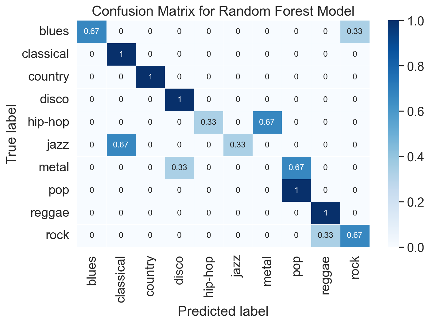
Feature importance
Let’s plot the feature importance from random forest classification.
import matplotlib.pyplot as plt
from matplotlib.pyplot import figure

importance = RF.feature_importances_
n = df_trimmed.columns[1:len(df.columns)]
im = pd.DataFrame({'data': importance,'names': n})
im2 = im.sort_values(by='data',ascending=False)
# plot feature importance
fig, ax = plt.subplots(figsize=(8, 5))
#figure(figsize=(10, 5))
plt.scatter(im2.names[0:9],im2.data[0:9],color='red')
plt.plot(im2.names[0:9],im2.data[0:9])
ax.set_title('10 strongest features')
plt.show()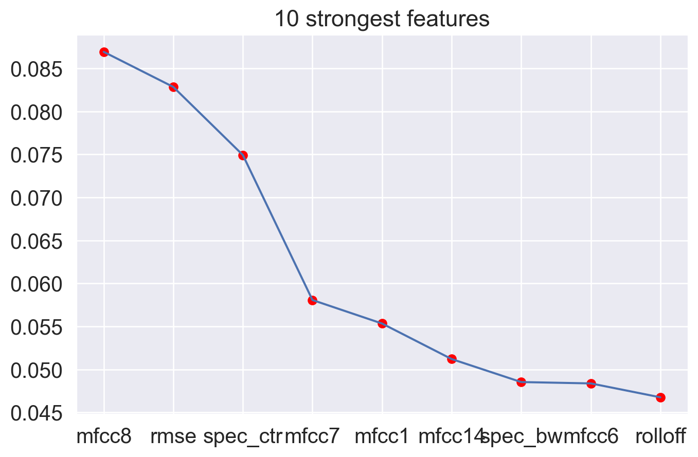
The plot show the best 10 features and the first four seem to bring greater benefit to the model.
Simplify model
What happens if we take the four best features and try building a simpler model with these features?
from sklearn.metrics import confusion_matrix, ConfusionMatrixDisplay

X2 = df_trimmed.filter(['mfcc8','rmse', 'spec_ctr', 'mfcc7'])

test_size = 0.30 # taking 70:30 training and test set
seed = 2022  # Random numbmer seeding for reapeatability of the code
X_train, X_test, y_train, y_test = train_test_split(X2, y, test_size=test_size, random_state=seed,stratify=y)

RF = RandomForestClassifier(n_estimators=1000, max_depth=10, random_state=seed).fit(X_train, y_train)
RF.predict(X_test)
# Make predictions for the test set
y_pred_test = RF.predict(X_test)
print(round(RF.score(X_test, y_test), 4))0.6333What do you think about the simplified model with 5 features? Is the model still good? You could look at the confusion to see what kind of mistakes the slimmer model starts to make.
There is concept call principle of parsimony or the idea behind that simpler models are more parsimonius than complex models, which stems from Occam’s razor. There are several statistical measures that assess the model fit and parsimoniousness (Akaike Information Criterion etc.). We are not entering into those calculations here but usually it is better to have a simple model and compromise the model accuracy a little bit than to gain few points in accuracy but having a complex model.
Summary
There numerous other algorithms to classify the materials, SVMs (Support Vector Machines), K-nearest neighbour models (KNNs), Neural networks, and many others.
We could have focussed more on features, their calculation, the summary measures, and subsets, but overall we achieved a good success with a small set of features. We have to remember that this is a mini-version of the original dataset. You are welcome to try how the full dataset would improve the results.
This process is pretty generic for all kinds of classification tasks, so the same procedure could be applied to prediction emotion categories, meter, instrumentation and other properties of music.
References
- Tzanetakis, G. & Cook, P. (2002). Musical genre classification of audio signals. IEEE Transactions on Speech and Audio Processing, 10(5), 293-302 doi:10.1109/TSA.2002.800560.