0.5 * (60 / 120)[1] 0.25This notebook demonstrates how to use R.
There are plenty of tools for data analysis and statistics available. I will only consider those that are open source and free to use as this is the only way to guarantee that people are able to access the tools. Sadly some fine tools such as SPSS, JMP, Minitab, SAS, or Stata don’t fulfil these principles. R and RStudio, JASP, Jamovi and Python (made better with libraries such as scipy) and some others are free and open source software that have become common research tools in empirical sciences. In addition to being free and easily available, they have excellent capacities to share the analysis workflow and some have tools to ensure replicability over years and different versions. I will focus on R in the statistical analysis and explain why I think this is a good option for analysis empirical data.
![]()
R is a versatile environment for analysing any data. It is interactive and suits well for casual exploration of data that comes in many different forms (numbers, text strings) and different shapes (long and wide data). What is even more important in R is that it is fundamentally based on scripts that serve as a blueprint of the analysis you have done and allows you, or anyone else, to replicate your analyses simply by running the same script. R is also:
incon,gm,hrep libraries) and datasets (MusicScienceData).Here is a quick tutorial for using R, but I would also recommend Getting Started with R and The Basics guides by the company who brings us RStudio (Posit).
The basic interface in R is called R console that will carry out commands as you type them. There are several ways to gain access to an R console. One way is to simply start R on your computer. The console looks something like this:

As an easy example, try using the console in R to calculate the duration in seconds of an eight note (or a quaver in the U.K.) in common time signature (4/4) when the tempo is quarter note = 120 beats per minute (BPM):
0.5 * (60 / 120)[1] 0.25The code boxes show R code typed into the R console. Anything followed by hashtag (#) is a comment and will not be interpreted by R. Here we see that one eight note is 0.25 seconds (or 250 ms if you want) in this tempo. We got this by remembering that one quarter note lasts for 60 / tempo in BPM seconds. And since eighth note is a half of a quarter note, we expressed this as 0.5 and multiplied (* ) this with the tempo expression (60/120). You would get the same result with 1/2 * 60/120. Or you could define the duration and tempo as an equation:
note <- 0.5
tempo <- 120
dur_in_seconds <- note * 60 / tempo  # Calculate
print(dur_in_seconds * 1000)   # Convert to milliseconds
[1] 250This example demonstrates that there are several ways of doing calculations in R. In the last example we tried to be clear about the operations and defined variables (note and tempo) and used them to calculate the duration of the note and finally to transform the value into milliseconds.
RStudio is a sleek and interactive integrated development environment (IDE) that offers a number of great features to use R efficiently as it offers the console, and panes for folders, help files, an index of what it is the memory, and a separate window for plots.

There are three main panes in RStudio. The left pane shows the R console. On the right, the top pane includes tabs such as Environment and History, while the bottom pane shows five tabs: File, Plots, Packages, Help, and Viewer.
Scripts are a collection of commands that can be edited with a text editor and executed in R.
To start a new script, you can click on File, then New File, then R Script. This starts a new pane on the left and it is here where you can start writing your script. This will contain your analysis. By documenting the analysis in the script, you, or anyone else, can replicate the steps in the script very easily and get the same results afterwards just by running the script.
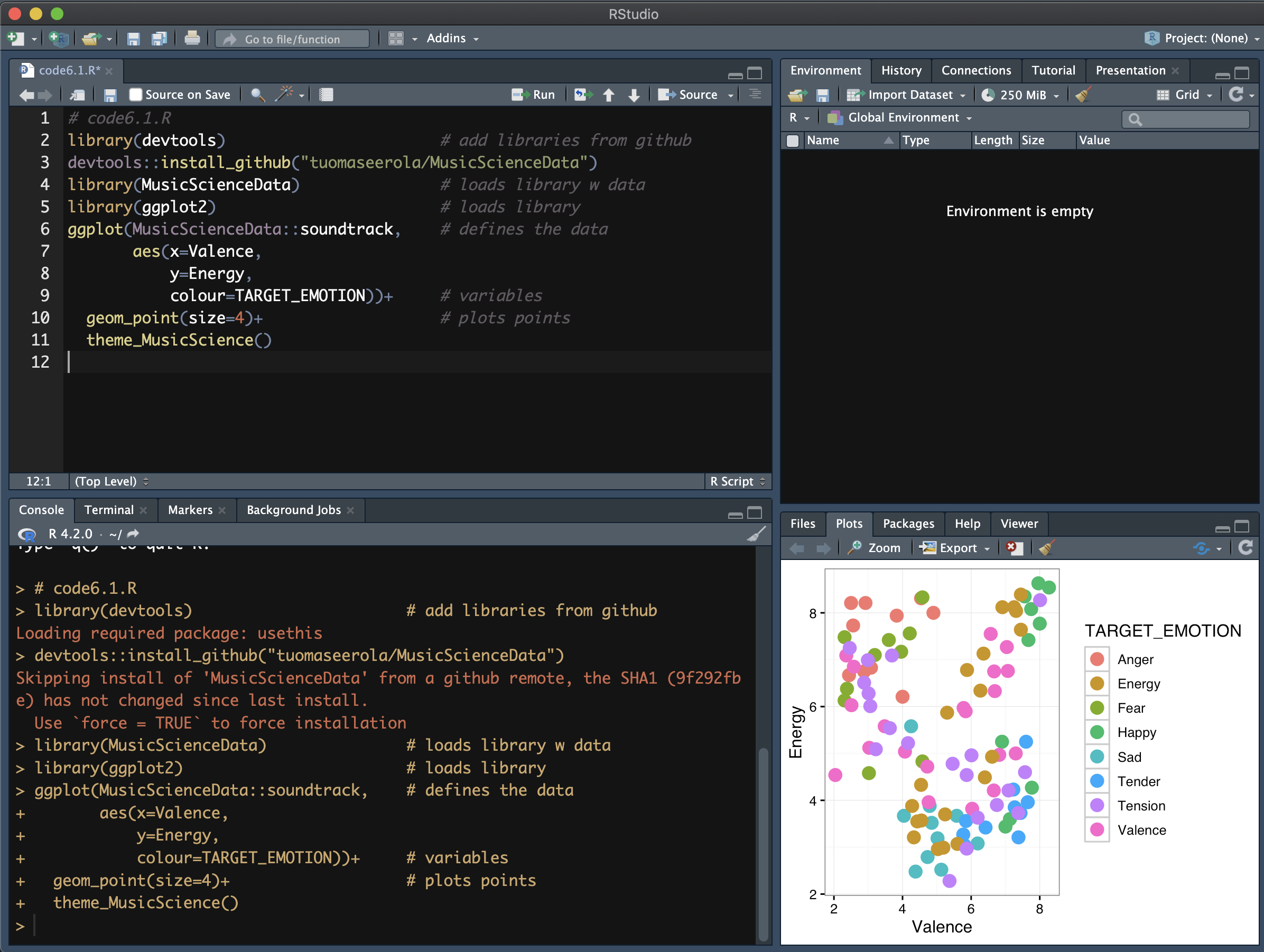
RStudio helps to make the code more readable and easy to use by making different parts of the code in different colour and the indentation is automatically modified as you write the code. It will also close the parenthesis and suggest the variable names as you go along, and warn if a line of code contains an error. If we look at our new script, we first need to give it a name. A good practice is to name scripts in a descriptive fashion, use lower case letters, avoid spaces, only to use hyphens to separate words, and then followed by the suffix .R. We will call this script code6.1.R. This one will grab data from a published dataset of emotions expressed by film soundtracks and plot the rated mean valence and energy of each track.
See Chapter7.R R code at https://tuomaseerola.github.io/emr/ site.
# code6.1.R
#library(devtools)                       # add libraries from github
#devtools::install_github("tuomaseerola/MusicScienceData")
library(MusicScienceData)               # loads library w data
library(ggplot2)                        # loads library
ggplot(MusicScienceData::soundtrack,    # defines the data
       aes(x=Valence,
           y=Energy,
           colour=TARGET_EMOTION))+     # variables
  geom_point(size=4)+                   # plots points
  theme_MusicScience()                  # applies style
Let’s review this script. The first four lines of code in an R script are used to load the libraries that are needed. Here we load the data from soundtrack study, which is part of the MusicScienceData library. As an example, we will make a graph showing the position of 110 music excerpts in terms of their rated Valence and Energy. Once you have copied or typed the code above, you can run it by executing the code by clicking on the Run button on the upper right side of the editing pane.
Once you run the code, you will see it appear in the R console and, in this case, the generated plot appears in the plots console. The plot console has a useful interface that permits you to click back and forward across different plots, zoom in to the plot, or save the plots as files. I recommend learning to save the plots as graphics directly in the script so that it is easier to control their size (width and height, and resolution) and type (pdf, tiff, or png), and to replicate the identical plots afterwards.
To run one line at a time instead of the entire script, you can use Control-Enter on Windows and command-return on the Mac Os.
R has thousands of libraries available that offer data, libraries and functions. Not everybody needs all these functionalities, so R offers these as packages that are easy to install within R. We will need a few of these so let’s see how this works.
In RStudio, the Tools tab contains an option to install packages. We can load a package into our R sessions using the library function:
library(ggplot2)If this command gives you an error, you probably do not have this fabulous plotting library installed in your R yet. This can be fixed by typing:
install.packages("ggplot2")After installation, you still need to make the library active in your session by invoking the library command described earlier. Different examples in this book will utilise different libraries. We only install the libraries once, because they remain installed and only need to be loaded with the library command.
The library where many examples come from, MusicScienceData, needs to be installed with the following code. This is because I have only released that library at Github for easier development, and R is not able to find it unless you have this extra package called devtools installed.
install.packages("devtools") # add libraries from github
devtools::install_github("tuomaseerola/MusicScienceData")