Show the code
import numpy as np
import librosa
import librosa.display
import IPython.display as ipd
from matplotlib import pyplot as plt import numpy as np
import librosa
import librosa.display
import IPython.display as ipd
from matplotlib import pyplot as plt x, sr = librosa.load('data/help.mp3', offset=1.05, duration=10.087)
ipd.display(ipd.Audio(data=x, rate=sr))fig, ax = plt.subplots(nrows=1,figsize=(7.5, 2.75))
librosa.display.waveshow(x, sr=sr, ax=ax, color='indigo')
ax.set_title("Waveform")
ax.set_xlabel("Time (s)")
ax.set_ylabel("Amplitude")
ax.set_xticks(range(0, 11, 1))
ax.set_xlim([0, 10])
ax.grid()
fig.tight_layout()
plt.show()
fig, ax = plt.subplots(nrows=1, figsize=(7.5, 2.75))
rms = librosa.feature.rms(y=x)                 # Extra dynamics (RMS)
db = librosa.amplitude_to_db(rms, ref=np.max)   # Convert into dB. Note that this is a relative measure (loudest is now 0)
times = librosa.times_like(rms)

ax.plot(times, db[0], color='darkblue')
ax.set_title("Loudness")
ax.set_ylim([-15,0])
ax.set_ylabel("Decibel")
ax.set_xlabel("Time (s)")
ax.set_xticks(range(0, 11, 1))
ax.set_xlim([0, 10])
ax.grid()
fig.tight_layout()
plt.show()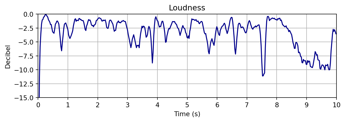
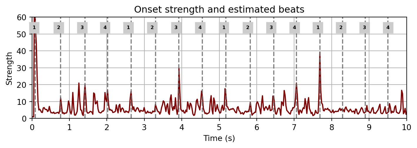
fig, ax = plt.subplots(nrows=1, figsize=(7.5, 2.75))


onset_subbands = librosa.onset.onset_strength_multi(y=x,
                                                    sr=sr,
                                                    channels=[0, 32, 64, 96, 128])

onset_subbands_s = sum(onset_subbands, 1)
ax.plot(times, onset_subbands_s, 'maroon')

tempo, beats = librosa.beat.beat_track(y=x, sr=sr, trim=False)
plt.vlines(times[beats], 0, onset_subbands_s.max(), color='0.40', alpha=0.80,
           linestyle='--', label='Beats')

o_env = librosa.onset.onset_strength(y=x, sr=sr)
times = librosa.times_like(o_env, sr=sr)
onset_frames = librosa.onset.onset_detect(onset_envelope=o_env, sr=sr)

ax.set_title("Onset strength and estimated beats")
ax.set_ylabel("Strength")
ax.set_xlabel("Time (s)")
ax.set_ylim([0, 60])
ax.set_xticks(range(0, 11, 1))
ax.set_xlim([0, 10])
ax.grid()
fig.tight_layout()

data = np.loadtxt('data/Help_beats.csv')
ann_time = data[0:16, 0]-1.05
ann_label = data[0:16, 1]
for x in range(16):
    ax.text(ann_time[x], 53, int(ann_label[x]), size=6,
            backgroundcolor='0.8', weight='bold', ha='center')

plt.show()