if (!require(devtools)) install.packages("devtools",
  repos = "http://cran.us.r-project.org")
devtools::install_github("tuomaseerola/inconMore")Ch. 3 – Historic profiles
Load libraries
Load or install necessary R packages.
library(inconMore)
library(ggplot2, quietly = TRUE)
library(tidyverse, quietly = TRUE)
options(repr.plot.width = 6, repr.plot.height = 4) # Default plot size for Colab
Code 3.1
Frequency of intervals in Bach sinfonias (bars) and ratings of consonance of the intervals (lines, from Bowling, Purves & Gill, 2018). Interval frequencies recreated from Huron 2001.
IV<-c("P1","m2","M2","m3","M3","P4","TT","P5","m6","M6","m7","M7","P8")
Frequency <- c(15,7,26,87,58,50,35,52,65,88,32,3,23)/100 # approx. from Huron 2001, p. 20
library(inconMore) # Let's use more recent data
a <- inconMore::bowl18 # Bowling et al., 2018 ratings for 12 intervals
Consonance <- scales::rescale(c(NA,a$rating[1:12]),to = c(0,1)) # No unison
df <- data.frame(IV,Consonance,Frequency)
df$Nro <- 1:13
Plot both.
g1 <- ggplot(df)  +
  geom_bar(aes(x=Nro, y=Frequency),stat="identity", fill="gray40",colour='black')+
  geom_line(aes(x=Nro, y=Consonance),stat="identity", group=1,linewidth=1.25,colour="gray80",alpha=0.80)+
  geom_point(aes(x=Nro, y=Consonance),stat="identity", group=1,size=3,alpha=0.80)+
  theme_bw()+
  xlab('Interval')+
  ylab('Normalized Freq./Consonance')+
  scale_x_continuous(breaks = seq(1,13,by=1),labels = IV,expand = c(0.01,0.01))+
  scale_y_continuous(breaks = seq(0,1,by=0.25),expand = c(0.01,0.01),limits = c(0,1))
g1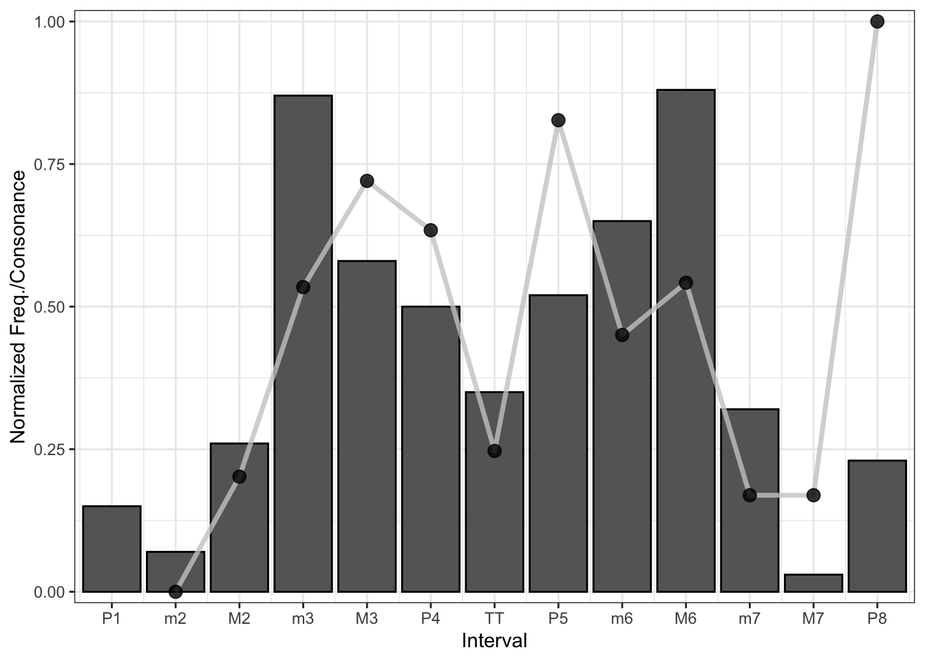
References
- Bowling, D. L., Purves, D., & Gill, K. Z. (2018). Vocal similarity predicts the relative attraction of musical chords. Proceedings of the National Academy of Sciences, 115(1), 216–221.
- Huron, D. (2001). Tone and voice: A derivation of the rules of voice-leading from perceptual principles. Music Perception, 19(1), 1–64.