Show the code
import numpy as np
import librosa
import librosa.display
from matplotlib import pyplot as plt The instrument samples are taken from McGill University Master Samples (MUMS, Opolko & Wapnick, 2006), polished by Eerola and Ferrer (2008) and used in subsequent experiments (Eerola et al., 2012).
import numpy as np
import librosa
import librosa.display
from matplotlib import pyplot as plt x, sr = librosa.load('data/63.wav')
stft = np.abs(librosa.stft(x))
freqs = librosa.fft_frequencies(sr=sr)
f0, voiced_flag, voiced_probs = librosa.pyin(x, fmin=librosa.note_to_hz('C2'),
fmax=librosa.note_to_hz('C7'))
f = np.nanmedian(f0) # Get the Hz of the F0 for nice labels
n = librosa.hz_to_note(f) # Convert Hz to note name
print(n)
X = np.arange(f, f*10, f)
fig, ax = plt.subplots(nrows=2, ncols=1, figsize=(8.0, 5.0))
# 1. Spectrum of a tone
# collapse across time and plot a spectrum
Dmean = stft.mean(axis=1)/max(stft.mean(axis=1))
ax[0].plot(freqs, Dmean, color='blue')
ax[0].set_title("Violin Spectrum")
ax[0].set(xlim=[130, X.max()])
ax[0].set_ylabel("Norm. Ampl.")
ax[0].set_xlabel("Frequency (Hz)")
ax[0].grid()
ax[0].set_xticks(X)
# calculate spectral centroid and plot it
centroid = librosa.feature.spectral_centroid(y=x, sr=sr)
centroidM = centroid.mean()
print(centroidM.round(0))
centroidM_label = "Centroid " + str(int(centroidM.round(0)))+" Hz"
ax[0].annotate("", xy=(130, 0.75), xycoords='data', xytext=(centroidM, 0.75),
arrowprops=dict(arrowstyle="<|-", connectionstyle="arc3",
color="0.3"), size=4)
ax[0].annotate("", xy=(centroidM, 0.75), xycoords='data',
xytext=(X.max(), 0.75),
arrowprops=dict(arrowstyle="-|>", connectionstyle="arc3",
color="0.3"), size=4)
ax[0].text(centroidM-120, 0.83, centroidM_label, size=10, color='0.2')
# Envelope
rms = librosa.feature.rms(y=x, frame_length=2048, hop_length=512)
times = librosa.times_like(rms)
ax[1].plot(times, rms[0], color='red')
librosa.display.waveshow(x, sr=sr, ax=ax[1], color='0.75', max_points=3000)
ax[1].grid()
ax[1].set(ylim=[-0.25, 0.25])
ax[1].text(0.25, 0.17, "A", size=12, color='0.2')
ax[1].text(1.20, 0.17, "S", size=12, color='0.2')
ax[1].text(1.85, 0.17, "D", size=12, color='0.2')
ax[1].annotate("", xy=(0.00, 0.15), xycoords='data', xytext=(0.50, 0.15),
arrowprops=dict(arrowstyle="|-|", connectionstyle="arc3",
color='0.2'), size=4)
ax[1].annotate("", xy=(0.50, 0.15), xycoords='data', xytext=(1.79, 0.15),
arrowprops=dict(arrowstyle="|-|", connectionstyle="arc3",
color='0.2'), size=4)
ax[1].annotate("", xy=(1.79, 0.15), xycoords='data', xytext=(2.0, 0.15),
arrowprops=dict(arrowstyle="|-|", connectionstyle="arc3",
color='0.2'), size=4)
ax[1].set_ylabel("Amplitude")
ax[1].set_title("Violin Envelope")
ax[1].set_xlabel("Time (s)")
fig.tight_layout()
plt.show()D♯4
1623.0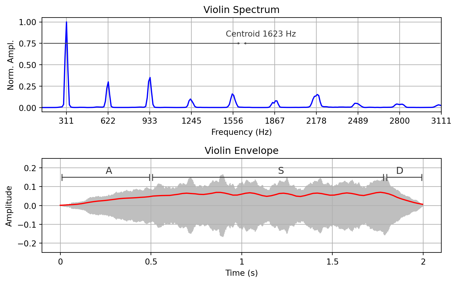
x, sr = librosa.load('data/24.wav')
stft = np.abs(librosa.stft(x))
freqs = librosa.fft_frequencies(sr=sr)

f0, voiced_flag, voiced_probs = librosa.pyin(x, fmin=librosa.note_to_hz('C2'), fmax=librosa.note_to_hz('C7'))
f=np.nanmedian(f0)        # Get the Hz of the fundamental frequency for nice labels
n=librosa.hz_to_note(f)  # Convert Hz to note name

X=np.arange(f,f*10,f)

fig, ax = plt.subplots(nrows=2, ncols=1, figsize=(8.0, 5.0))

# collapse across time and plot a spectrum representation (energy across frequencies)
Dmean=stft.mean(axis=1)/max(stft.mean(axis=1))
ax[0].plot(freqs,Dmean,color='blue')
#ax[0].label_outer()
#ax[0].set_title("Spectrum")
ax[0].set(xlim=[130, X.max()])
ax[0].set_ylabel("Norm. Ampl.")
ax[0].set_xlabel("Frequency (Hz)")
ax[0].grid()
ax[0].set_xticks(X)
ax[0].set_title("Clarinet Spectrum")

# calculate spectral centroid and plot it
centroid = librosa.feature.spectral_centroid(y=x, sr=sr)
centroidM = centroid.mean()
print(centroidM.round(0))
centroidM_label = "Centroid " + str(int(centroidM.round(0)))+" Hz"
ax[0].annotate("",xy=(130, 0.75), xycoords='data',xytext=(centroidM, 0.75), arrowprops=dict(arrowstyle="<|-",connectionstyle="arc3",color="0.3"),size=4)
ax[0].annotate("",xy=(centroidM, 0.75), xycoords='data',xytext=(X.max(), 0.75), arrowprops=dict(arrowstyle="-|>",connectionstyle="arc3",color="0.3"),size=4)
ax[0].text(centroidM-120,0.83,centroidM_label,size=10,color='0.2')

rms=librosa.feature.rms(y=x,frame_length=2048,hop_length=512)                 # Extra dynamics (RMS)
times = librosa.times_like(rms)
ax[1].plot(times, rms[0],color='red')

librosa.display.waveshow(x, sr=sr, ax=ax[1],color='0.75',max_points=3000)
ax[1].grid()
ax[1].set(ylim=[-0.25, 0.25])

ax[1].text(0.00,0.17,"A",size=12,color='0.2')
#ax[0,1].text(0.50,0.99,"D",size=15)
ax[1].text(0.90,0.17,"S",size=12,color='0.2')
ax[1].text(1.85,0.17,"D",size=12,color='0.2')
ax[1].annotate("",xy=(0.00, 0.15), xycoords='data',xytext=(0.07, 0.15),arrowprops=dict(arrowstyle="|-|",connectionstyle="arc3",color='0.2'),size=4)
#ax[0,1].annotate("",xy=(0.05, 0.14), xycoords='data',xytext=(0.20, 0.14),arrowprops=dict(arrowstyle="<->",connectionstyle="arc3"),size=15)
ax[1].annotate("",xy=(0.07, 0.15), xycoords='data',xytext=(1.77, 0.15),arrowprops=dict(arrowstyle="|-|",connectionstyle="arc3",color='0.2'),size=4)
ax[1].annotate("",xy=(1.77, 0.15), xycoords='data',xytext=(2.0, 0.15),arrowprops=dict(arrowstyle="|-|",connectionstyle="arc3",color='0.2'),size=4)
ax[1].set_ylabel("Amplitude")
ax[1].set_xlabel("Time (s)")
ax[1].set_title("Clarinet Envelope")

fig.tight_layout()
plt.show()
1701.0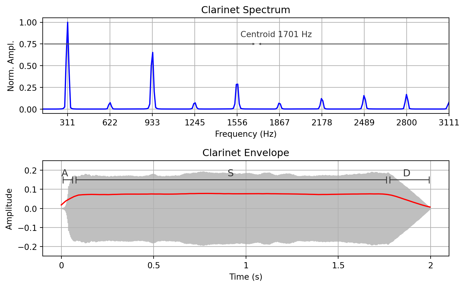
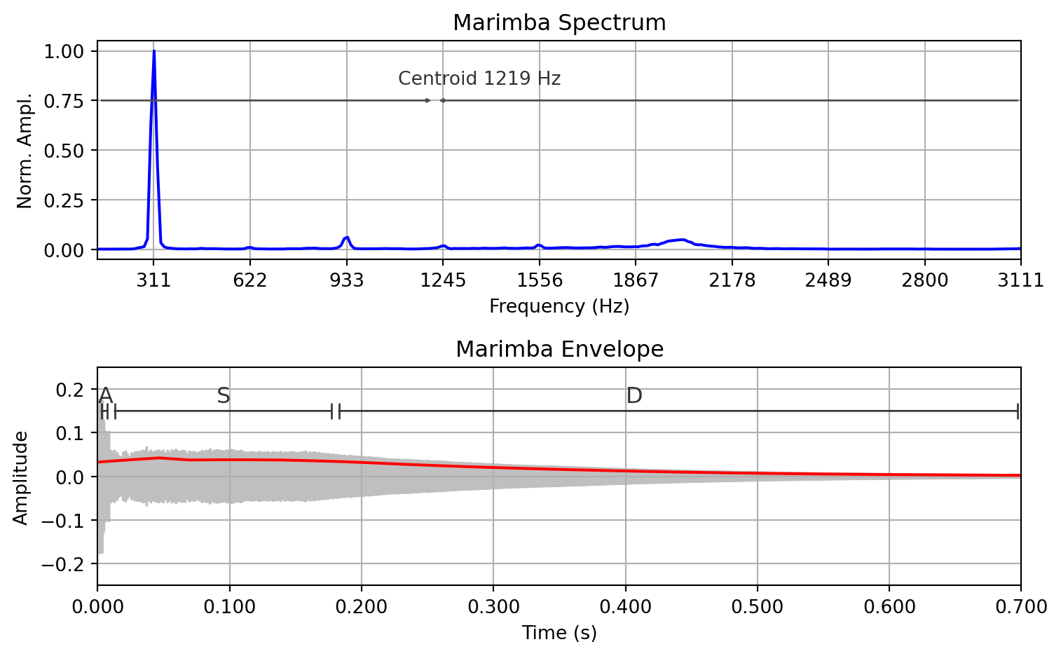
x, sr = librosa.load('data/90.wav')

stft = np.abs(librosa.stft(x))
freqs = librosa.fft_frequencies(sr=sr)

f0, voiced_flag, voiced_probs = librosa.pyin(x, fmin=librosa.note_to_hz('C2'), fmax=librosa.note_to_hz('C7'))
f=np.nanmedian(f0)        # Get the Hz of the fundamental frequency for nice labels
n=librosa.hz_to_note(f)  # Convert Hz to note name
print(n)
X=np.arange(f,f*10,f)

fig, ax = plt.subplots(nrows=2, ncols=1, figsize=(8.0, 5.0))


# collapse across time and plot a spectrum representation (energy across frequencies)
Dmean=stft.mean(axis=1)/max(stft.mean(axis=1))
ax[0].plot(freqs,Dmean,color='blue')
ax[0].set_title("Marimba Spectrum")
ax[0].set(xlim=[130, X.max()])
ax[0].set_ylabel("Norm. Ampl.")
ax[0].set_xlabel("Frequency (Hz)")
ax[0].grid()
ax[0].set_xticks(X)

# calculate spectral centroid and plot it
centroid = librosa.feature.spectral_centroid(y=x, sr=sr)
centroidM = centroid.mean()
print(centroidM.round(0))
centroidM_label = "Centroid " + str(int(centroidM.round(0)))+" Hz"
ax[0].annotate("",xy=(130, 0.75), xycoords='data',xytext=(centroidM, 0.75), arrowprops=dict(arrowstyle="<|-",connectionstyle="arc3",color="0.3"),size=4)
ax[0].annotate("",xy=(centroidM, 0.75), xycoords='data',xytext=(X.max(), 0.75), arrowprops=dict(arrowstyle="-|>",connectionstyle="arc3",color="0.3"),size=4)
ax[0].text(centroidM-120,0.83,centroidM_label,size=10,color='0.2')

rms=librosa.feature.rms(y=x,frame_length=2048,hop_length=512)
times = librosa.times_like(rms)
ax[1].plot(times, rms[0],color='red')
librosa.display.waveshow(x, sr=sr, ax=ax[1],color='0.75',max_points=3000)
ax[1].grid()
ax[1].set(ylim=[-0.25, 0.25])
ax[1].set(xlim=[0, 0.70])

ax[1].text(0.00,0.17,"A",size=12,color='0.2')
ax[1].text(0.09,0.17,"S",size=12,color='0.2')
ax[1].text(0.40,0.17,"D",size=12,color='0.2')
ax[1].annotate("",xy=(0.00, 0.15), xycoords='data',xytext=(0.01, 0.15),arrowprops=dict(arrowstyle="|-|",connectionstyle="arc3",color='0.2'),size=4)
ax[1].annotate("",xy=(0.01, 0.15), xycoords='data',xytext=(0.18, 0.15),arrowprops=dict(arrowstyle="|-|",connectionstyle="arc3",color='0.2'),size=4)
ax[1].annotate("",xy=(0.18, 0.15), xycoords='data',xytext=(0.70, 0.15),arrowprops=dict(arrowstyle="|-|",connectionstyle="arc3",color='0.2'),size=4)
ax[1].set_ylabel("Amplitude")
ax[1].set_title("Marimba Envelope")
ax[1].set_xlabel("Time (s)")

fig.tight_layout()
plt.show()
D♯4
1219.0