Show the code
import pandas as pd
import numpy as np
import spotipy
from spotipy.oauth2 import SpotifyClientCredentialsThis code requires that the user supplements their own client_id and client_secret which can be obtained after registering to developer account for Spotify API. The code will not run without these. However, the visualisation part of the code works with the save data (data/top_n_track_features2.csv).
import pandas as pd
import numpy as np
import spotipy
from spotipy.oauth2 import SpotifyClientCredentialsclient_id = 'YOUR_CLIENT_ID_HERE'
client_secret = 'YOUR_SECRET_KEY_HERE'
sp = spotipy.Spotify(auth_manager=SpotifyClientCredentials(client_id=client_id,
client_secret=client_secret))
results = sp.search(q='The Beatles', limit=20)
for idx, track in enumerate(results['tracks']['items']):
print(idx, track['name'])
track = results['tracks']['items'][18] # help is 18
print(track['name'])
print(track['href'])
print(track['popularity'])
print("===========PREVIEW===========")
print(track['preview_url'])
print("===========PREVIEW===========")
a = sp.audio_features(track['id'])
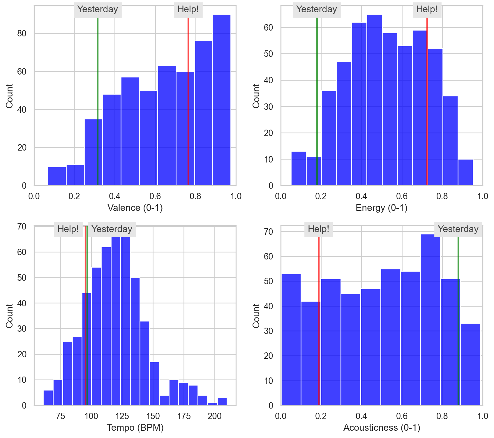
print(a[0]['valence']) # Help!: 0.763, Yesterday: 0.315
print(a[0]['energy']) # Help!: 0.725, Yesterday: 0.179
print(a[0]['tempo']) # Help!: 95.003, Yesterday: 96.53
print(a[0]['loudness']) # Help!: -7.576, Yesterday: -11.83
print(a[0]['acousticness']) # Help!: 0.188, Yesterday: 0.879
print("===========GENRE===========")
name = []
Tid = []
valence = []
energy = []
tempo = []
loudness = []
instrumentalness = []
acousticness = []
danceability = []
# get 500 tracks, 50 each time
offset_vals = np.arange(1, 500, 10)
for i in range(50):
results = sp.search(q='genre:pop & year:1964-1966', limit=10,
offset=offset_vals[i])
for idx, track in enumerate(results['tracks']['items']):
name.append(track['name'])
Tid.append(track['id'])
a = sp.audio_features(track['id'])
valence.append(a[0]['valence'])
energy.append(a[0]['energy'])
instrumentalness.append(a[0]['instrumentalness'])
acousticness.append(a[0]['acousticness'])
danceability.append(a[0]['danceability'])
tempo.append(a[0]['tempo'])
loudness.append(a[0]['loudness'])
print(i, ':', idx)
# Store in data frame and save to a file
df = pd.DataFrame({'valence': valence, 'energy': energy, 'tempo': tempo,
'acousticness': acousticness,
'loudness': loudness, 'id': Tid})
df.to_csv('data/top_n_track_features2.csv')import pandas as pd
import numpy as np
import seaborn as sns
from matplotlib import pyplot as plt
# Get data (from a previous process)
d = pd.read_csv('data/top_n_track_features2.csv')
# set graphic (seaborn) theme
sns.set_theme()
sns.set_style("whitegrid")
fig = plt.figure()
fig.set_figheight(8)
fig.set_figwidth(9)
# Define multiple plots
ax1 = plt.subplot2grid(shape=(2, 2), loc=(0, 0))
ax2 = plt.subplot2grid(shape=(2, 2), loc=(0, 1))
ax3 = plt.subplot2grid(shape=(2, 2), loc=(1, 0))
ax4 = plt.subplot2grid(shape=(2, 2), loc=(1, 1))
sns.histplot(x='valence', data=d, color='blue', ax=ax1)
ax1.set_xlabel('Valence (0-1)')
ax1.axes.axvline(0.763, color='red', linewidth=2, alpha=.7)
ax1.text(0.763, ax1.get_ylim()[1], "Help!", size=12, backgroundcolor='0.9',
ha="center", va="top", alpha=0.85)
ax1.axes.axvline(0.315, color='green', linewidth=2, alpha=.7)
ax1.text(0.315, ax1.get_ylim()[1], "Yesterday", size=12, backgroundcolor='0.9',
ha="center", va="top", alpha=0.85)
ax1.set_xlim([0, 1])
ax1.set_xticks(np.arange(0, 1.1, 0.20))
sns.histplot(x='energy', data=d, color='blue', ax=ax2)
ax2.set_xlabel('Energy (0-1)')
ax2.axes.axvline(0.725, color='red', linewidth=2, alpha=.7)
ax2.text(0.725, ax2.get_ylim()[1], "Help!", size=12, backgroundcolor='0.9',
ha="center", va="top", alpha=0.85)
ax2.axes.axvline(0.179, color='green', linewidth=2, alpha=.7)
ax2.text(0.179, ax2.get_ylim()[1], "Yesterday", size=12, backgroundcolor='0.9',
ha="center", va="top", alpha=0.85)
ax2.set_xlim([0, 1])
ax2.set_xticks(np.arange(0, 1.1, 0.20))
sns.histplot(x='tempo', data=d, color='blue', ax=ax3)
ax3.set_xlabel('Tempo (BPM)')
ax3.axes.axvline(95, color='red', linewidth=2, alpha=.7)
ax3.text(90, ax3.get_ylim()[1], "Help!", size=12, backgroundcolor='0.9',
ha="right", va="top", alpha=0.85)
ax3.axes.axvline(96.5, color='green', linewidth=2, alpha=.7)
ax3.text(100, ax3.get_ylim()[1], "Yesterday", size=12, backgroundcolor='0.9',
ha="left", va="top", alpha=0.85)
sns.histplot(x='acousticness', data=d, color='blue', ax=ax4)
ax4.set_xlabel('Acousticness (0-1)')
ax4.axes.axvline(0.188, color='red', linewidth=2, alpha=.7)
ax4.text(0.188, ax4.get_ylim()[1], "Help!", size=12, backgroundcolor='0.9',
ha="center", va="top", alpha=0.85)
ax4.axes.axvline(0.879, color='green', linewidth=2, alpha=.7)
ax4.text(0.879, ax4.get_ylim()[1], "Yesterday", size=12, backgroundcolor='0.9',
ha="center", va="top", alpha=0.85)
ax4.set_xlim([0, 1])
ax4.set_xticks(np.arange(0, 1.1, 0.20))
fig.tight_layout()
plt.show()