Minimal representation • onsetsync

What is the minimal amount of representation for the common functions? It depends on the function and the purpose of the analysis, but here we document three minimal cases: One with just pair of onsets, the same with a reference time (mean onset time), and an example with an external timing of the cycles.

Minimal example: Onsets of two instruments and a beat sub-division

We assume the minimal case will be two instruments playing together. Here we create 8 joint onsets tapping in isochrony around twice a second with a random variation. We also assume that there is a beat division representing common time (4 beats/cycle), although the existence of the beat sub-division (SD) does not need to reflect any particular cycle, it could also be just a sequence of numbers.

library(onsetsync)
set.seed(12345) # to create the same random variation every time
ex <- data.frame(SD = rep(1:4,2), 
                 instr1 = rep(0:7/2)+runif(8,min = -0.02,max=0.02), 
                 instr2 = rep(0:7/2) + runif(8,min = -0.02,max=0.02)
                 )
print(knitr::kable(ex))

SD	instr1	instr2
1	0.0088362	0.0091082
2	0.5150309	0.5195895
3	1.0104393	0.9813814
4	1.5154450	1.4860949
1	1.9982592	2.0094274
2	2.4866549	2.4800455
3	2.9930038	2.9956481
4	3.5003690	3.4984998

Here we have two instruments (instr1 and instr2) and a simple beat sub-division (SD). Note that beat sub-division do not need to be specific, it could be a column of numbers (you could create such a column with ex$SD <- 1:nrow(ex) if you only have onsets, nothing else). For the basic analysis of synchrony, this is already sufficient for the calculation of asynchronies.

d <- sync_sample_paired(ex,'instr1','instr2', beat = 'SD')
print(paste('Mean absolute asynchrony:', round(mean(abs(d$asynch*1000)),0),'ms'))

## [1] "Mean absolute asynchrony: 11 ms"

Minimal example with a reference time

Let’s add a reference time for a minimal representation that is required for plotting. Here we create a reference time which is the mean of the instrument onsets using add_isobeats() function.

ex1 <- add_isobeats(ex, instr = c("instr1","instr2"), beat = "SD")
print(knitr::kable(head(ex1,4)))

SD	instr1	instr2	Mean.Time
1	0.0088362	0.0091082	0.0089722
2	0.5150309	0.5195895	0.5173102
3	1.0104393	0.9813814	0.9959104
4	1.5154450	1.4860949	1.5007700

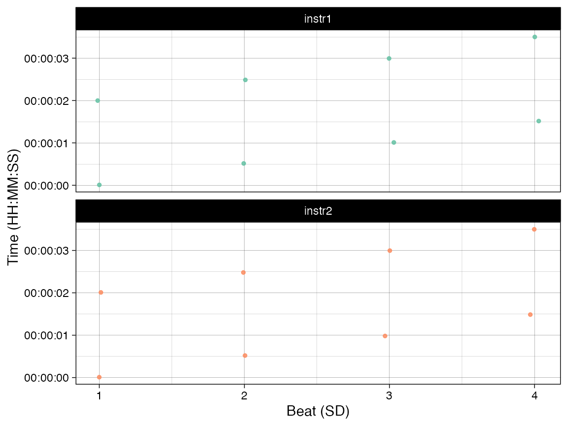
This representation (two instruments, beat sub-divisions, and a reference timing) is the minimal representation for many plotting functions (e.g., plot_by_beat()). The explicit reference time (Mean.Time) is used in plotting.

library(dplyr)
library(ggplot2)
g1 <- plot_by_beat(ex1, instr = c("instr1","instr2"), beat = "SD",virtual = 'Mean.Time')
g1

Minimal example with an external reference time (annotations of cycles)

Sometimes you might have independent information (through annotations) about the timing of the sub-divisions and how they relate to cycles. Let’s create this scenario and add Cycle information and timing (CycleTime).

ex2 <- cbind(ex, Cycle = c(rep(1,4),rep(2,4)), CycleTime=NA) # add cycle
ex2$CycleTime[seq(1, 8, by = 4)] <- seq(0, 2, by = 2) # add cycle time for beginnings
ex2 <- rbind(ex2,data.frame(Cycle = 3, SD = 1, # add beginning of the 3rd cycle
                            instr1 = 4, instr2 = 4, CycleTime = 4)) 
print(knitr::kable(ex2))

SD	instr1	instr2	Cycle	CycleTime
1	0.0088362	0.0091082	1	0
2	0.5150309	0.5195895	1	NA
3	1.0104393	0.9813814	1	NA
4	1.5154450	1.4860949	1	NA
1	1.9982592	2.0094274	2	2
2	2.4866549	2.4800455	2	NA
3	2.9930038	2.9956481	2	NA
4	3.5003690	3.4984998	2	NA
1	4.0000000	4.0000000	3	4

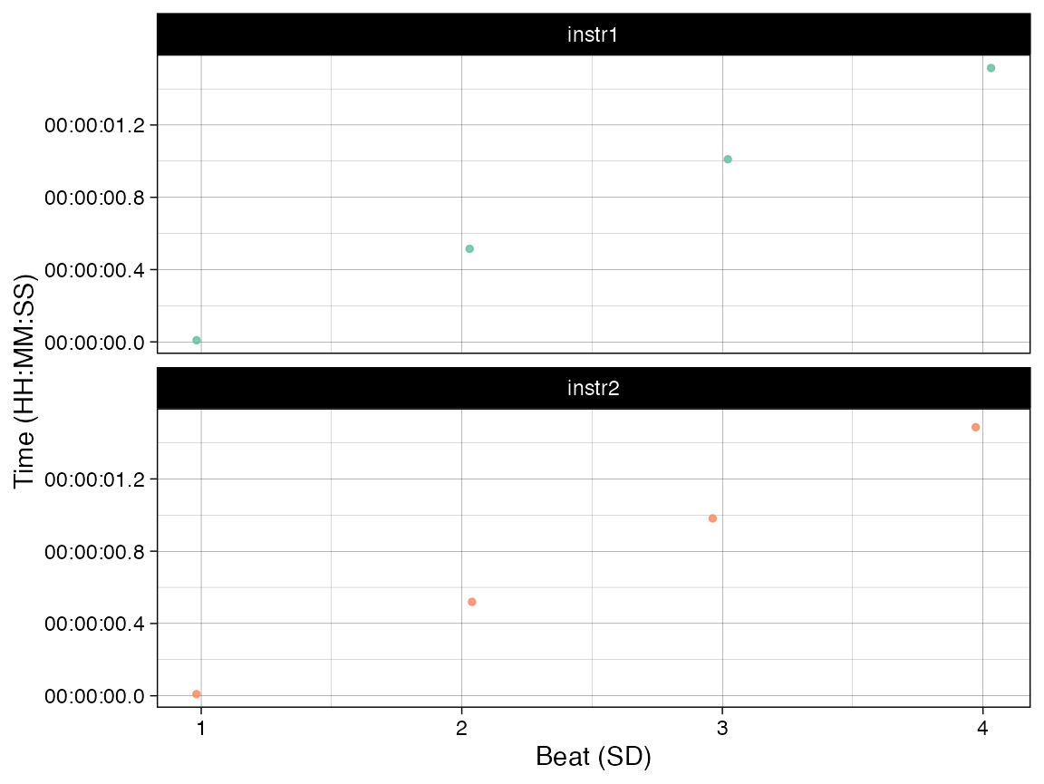
Now we add the timing of the onsets across beat sub-divisions (SD) based on this external CycleTime. The outcome of the add_isobeats() will now be called Iso.Time, although you can rename it with beatlabel option.

ex2 <- add_isobeats(ex2, instr = "CycleTime", beat = "SD")
print(knitr::kable(head(ex2,4)))

SD	instr1	instr2	Cycle	CycleTime	Iso.Time
1	0.0088362	0.0091082	1	0	0.0
2	0.5150309	0.5195895	1	NA	0.5
3	1.0104393	0.9813814	1	NA	1.0
4	1.5154450	1.4860949	1	NA	1.5

g2 <- plot_by_beat(ex2, instr = c("instr1","instr2"), beat = "SD", virtual = 'Iso.Time')
g2