Advanced topics

Synchrony between the instruments across beat subdivisions

In the first visualisation we already observed that asynchronies varied across beat subdivision (shown with respect to the equal subdivision) in the example with the tres and the guitar. Here we continue the analysis of the guitar and the tres and calculate the asynchrony between them across the beat subdivisions. The summary of the differences in milliseconds is contained in the output. This output reports the asynchrony between the instruments across the subdivisions and the provides an index of whether the mean differences are significantly different from zero. In other words, the summary shows in which beat subdivisions the two musicians are performing asynchronously in a consistent manner.

library(onsetsync)
library(ggplot2)
library(dplyr)
CSS_Song2 <- dplyr::select(onsetsync::CSS_IEMP[[2]],
  Piece, Section, Clave, Bass, Guitar, Tres, 
  SD, Cycle, Isochronous.SD.Time)

dn <- sync_execute_pairs(df = CSS_Song2,
  instruments = c("Guitar", "Tres"),
  beat = "SD")
print(knitr::kable(summarise_sync_by_pair(dn, bybeat = TRUE),
  digits = 2,caption = 'Asynchrony between tres and guitar 
  across beat sub-divisions.'))

Asynchrony between tres and guitar across beat sub-divisions.
Subdivision	N	M	SD	T	pval
1	48	5.03	21.87	1.60	>0.999
2	34	9.98	29.59	1.97	0.922
3	56	9.28	32.69	2.12	0.611
4	76	17.36	31.63	4.78	<0.001
5	52	10.11	23.25	3.13	0.046
6	26	8.77	27.32	1.64	>0.999
7	83	7.53	25.73	2.67	0.148
8	70	14.51	26.99	4.50	<0.001
9	44	17.53	18.86	6.17	<0.001
10	41	5.29	24.68	1.37	>0.999
11	29	13.80	25.34	2.93	0.106
12	70	19.51	29.22	5.59	<0.001
13	68	9.07	20.76	3.60	0.010
14	17	14.31	34.51	1.71	>0.999
15	68	7.44	21.44	2.86	0.089
16	71	24.72	26.69	7.81	<0.001

The output of Table 1 suggests that about half of the asynchronies in the subdivisions are statistically significant (and this includes a correction for multiple comparisons using the Bonferroni adjustment). Asynchronies over 10 ms tend to be statistically significant and these fall into beat subdivisions 4, 8, 9, 12, 13, and 16. Here we are using t-test as an arbitrary indicator of the differences since the assumption for the independence of the observations is not met since the two instruments are temporally not independent.

Calculation of asynchronies between parts depends on the number of comparable onsets (points at which both are playing on the same beat subdivision). This will be relatively high in music with a homophonic texture, and low in an interlocking or hocketing pattern where the musicians are playing on alternating beats. In Cuban salsa and son, some instruments play on most subdivisions (as with the guitar and the tres in this piece) while others are relatively sparse and may only coincide a few times per cycle. In this piece the clave plays on subdivisions 1, 4, 7, 11, 13 while the bass starts off playing on subdivisions 4, 5, 7, 13, 15; thus they coincide on subdivisions 4, 7 and 13 on most cycles and these subdivisions are the points at which we can calculate asynchronies. In sum, the number of joint onsets (onset occurring around the same beat) for each pair of instrument varies greatly. To keep the mean and standard deviations comparable, we can randomly sample an equal number of joint onsets for both instruments.

Synchrony across multiple performances

So far our analysis has considered synchrony within a single performance. We can also take several performances, choose the instrument pairings, and carry out the desired comparison, provided that this is conceptually meaningful and technically feasible (similar types of onset and annotation data are available). For this, we load five Cuban Son and Salsa performances that come with the library and run the same analysis as was done in prior examples using sync_sample_paired function across the performances.

corpus <- onsetsync::CSS_IEMP
D <- sync_sample_paired(corpus,"Guitar","Tres", beat="SD")
D <- D$asynch
D$asynch_abs <- abs(D$asynch)*1000
print(plot_by_dataset(D,"asynch_abs","name", box = TRUE))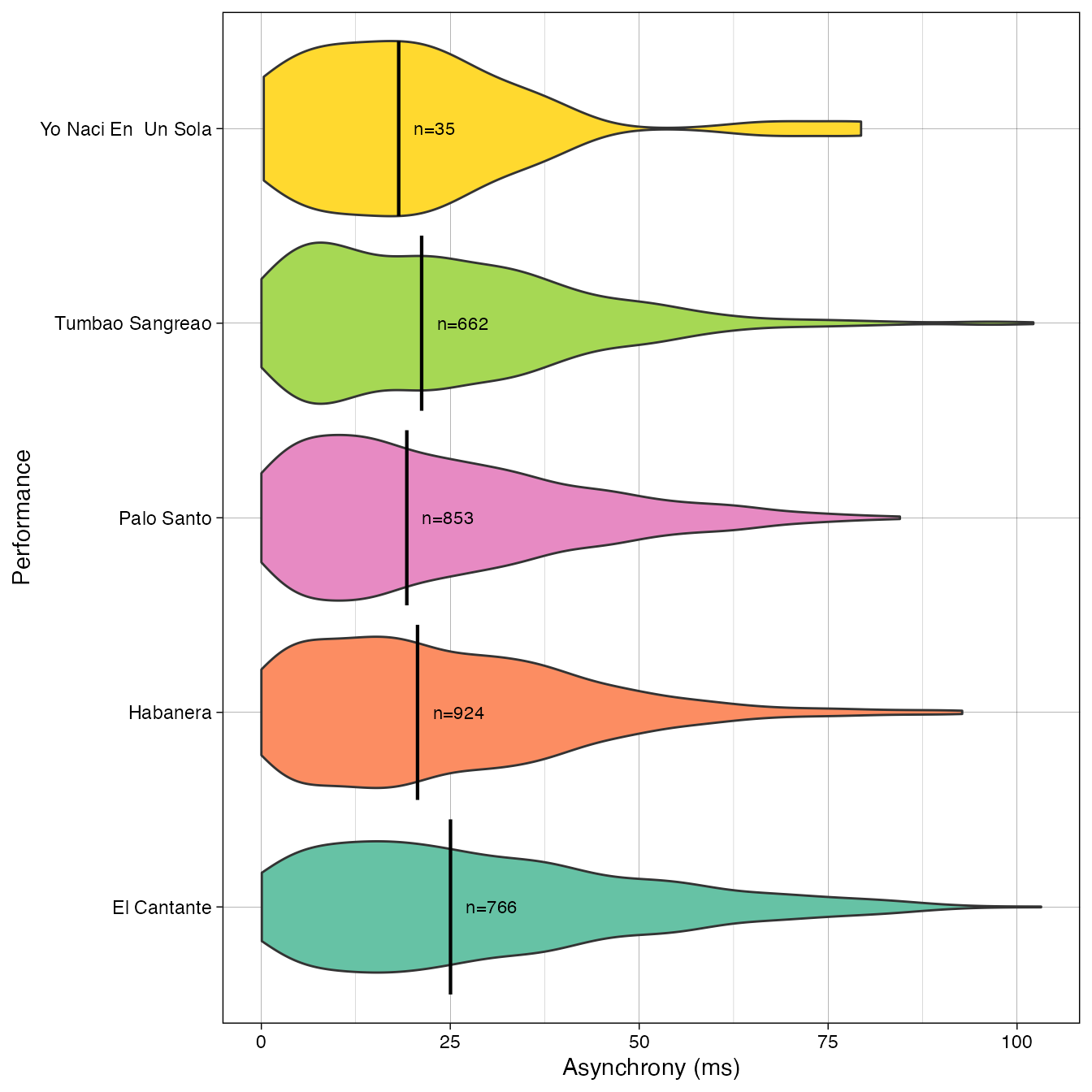

Figure 1. Absolute asynchronies between the guitar and the tres in five performances within the CSS_IEMP dataset.

We can create a simple violin plot of the combined data ignoring the beat sub-divisions (Figure 1). All further analyses and summaries are then also possible.

Figure 1 suggests that the asynchrony of 13 ms between the tres and the guitar we saw in the analysis of is largely in line with the overall asynchrony between the same instruments in the other instruments (overall mean asynchrony in all 5 pieces is 17 ms) although our example piece () shows the tightest synchrony in these examples.

Synchrony with other variables

It is relatively straightforward to explore whether synchrony is linked with another variable. For example, the precision of synchrony could change when the tempo of the performance is faster or slower. Or synchrony might be influenced by the dynamics or note density in a specific section. As an example, we illustrate synchrony across the time and tempo. As tempo is commonly defined by the beats per minute (BPM), we use the cycle information to convert the isochronous beat times to BPM.

CSS_Song2 <- CSS_Song2 %>%
  group_by(Cycle) %>%
  mutate(Tempo = 240/(max(Isochronous.SD.Time) - 
                        min(Isochronous.SD.Time))) %>%
  ungroup()

d2 <- sync_sample_paired(CSS_Song2,"Tres","Guitar", 
                         beat = "Tempo")
d3 <- sync_sample_paired(CSS_Song2,"Tres","Guitar", 
                         beat = "Isochronous.SD.Time")
tmp <- data.frame(asynch = d2$asynch*1000, 
                  Tempo = d2$beatL, 
                  Time = d3$beatL)
print(plot_by_var_time(df = tmp,
  var1 = "Time",
  var2 = "asynch",
  var3 = "Tempo",
  ylabel = "Asynchrony (ms)"))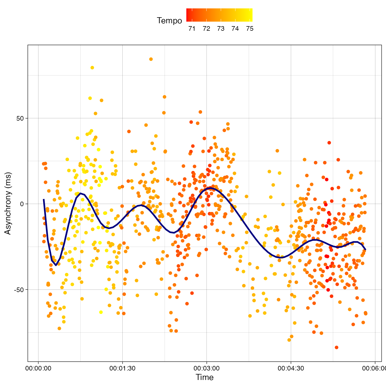

Figure 2. Asynchrony between the tres and the guitar (Y-axis) across time (X-axis) and tempo (illustrated with marker colors).

As Figure 2 shows, synchrony fluctuates across time but these fluctuations do not seem to be directly related to the underlying tempo changes, although the last minute and half is performed slightly slower (\(\approx71\) BPM) and the guitar is approximately 20 ms ahead of the tres.

Back to Documentation