Analysis of periodicity
analysis_of_periodicity.RmdAnalysis of periodicity
We can also explore the periodic nature of the instrument onset times without reference to the metrical structure. Functions described in this part may in fact be particularly useful in other musical genres which do not exhibit a clear metrical structure; nonetheless they are illustrated here using the example used in the previous analyses.
Let’s take the guitar onsets in the first example () and define an extract of 5 seconds starting from 1 minute mark. We know from the previous analyses that guitar keeps a fairly steady beat, separated by about 0.25 seconds while leaving out some beats.
library(onsetsync)
library(ggplot2)
CSS_Song2 <- dplyr::select(onsetsync::CSS_IEMP[[2]],
  Piece, Section, Clave, Bass, Guitar, Tres,
  SD, Cycle, Isochronous.SD.Time)
extract <- dplyr::filter(CSS_Song2, Guitar >= 60 & Guitar < 65)
fig2A <- gaussify_onsets(extract$Guitar, wlen = 0.2, plot = TRUE)
For the periodicity analyses, we want to transform the discrete onsets to continuous time representation with an uniform sampling rate. This is done with the function. This makes the comparisons of the models easier and allows us to handle time more explicitly. From this new continuous representation, we can estimate the periodicity of the guitar strokes by using different methods; Here we demonstrate (a) a simple time difference method, (b) method based on autocorrelation, and (c) fast fourier transform. We constrain the frequency to a range of 0.05 to 0.50 seconds. After the extraction of periodicity with function, we plot the estimated frequency curves (Figure 1).
frq_range <- c(0.05,0.50)
fig2B <- periodicity(extract, instr = "Guitar",
  freq_range=frq_range, method = "diff", title = "Difference")
fig2C <- periodicity(extract, instr="Guitar",
  freq_range=frq_range, method = "acf",title = "Autocorrelation")
fig2D <- periodicity(extract, instr="Guitar",
  freq_range=frq_range, method = "per",title = "FFT")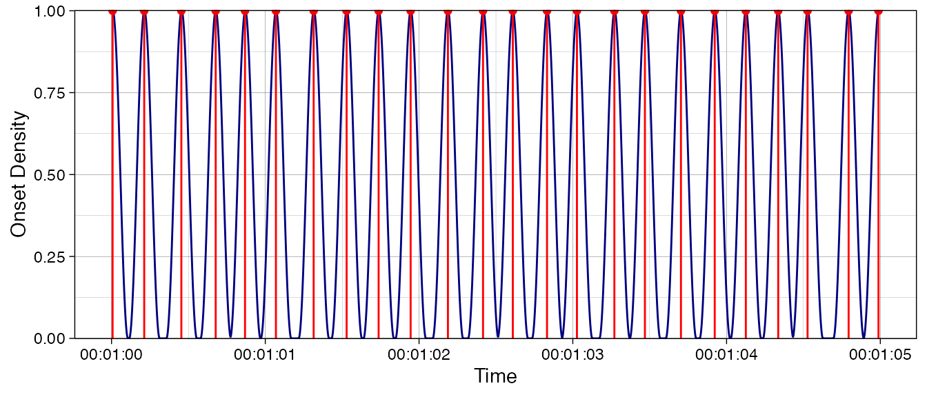
Figure 1. Periodicity analysis of a 5-second extract of guitar playing in Cuban son. Panel A shows the onsets (red) and the conversion into gaussian distributions (blue) for a continuous representation.
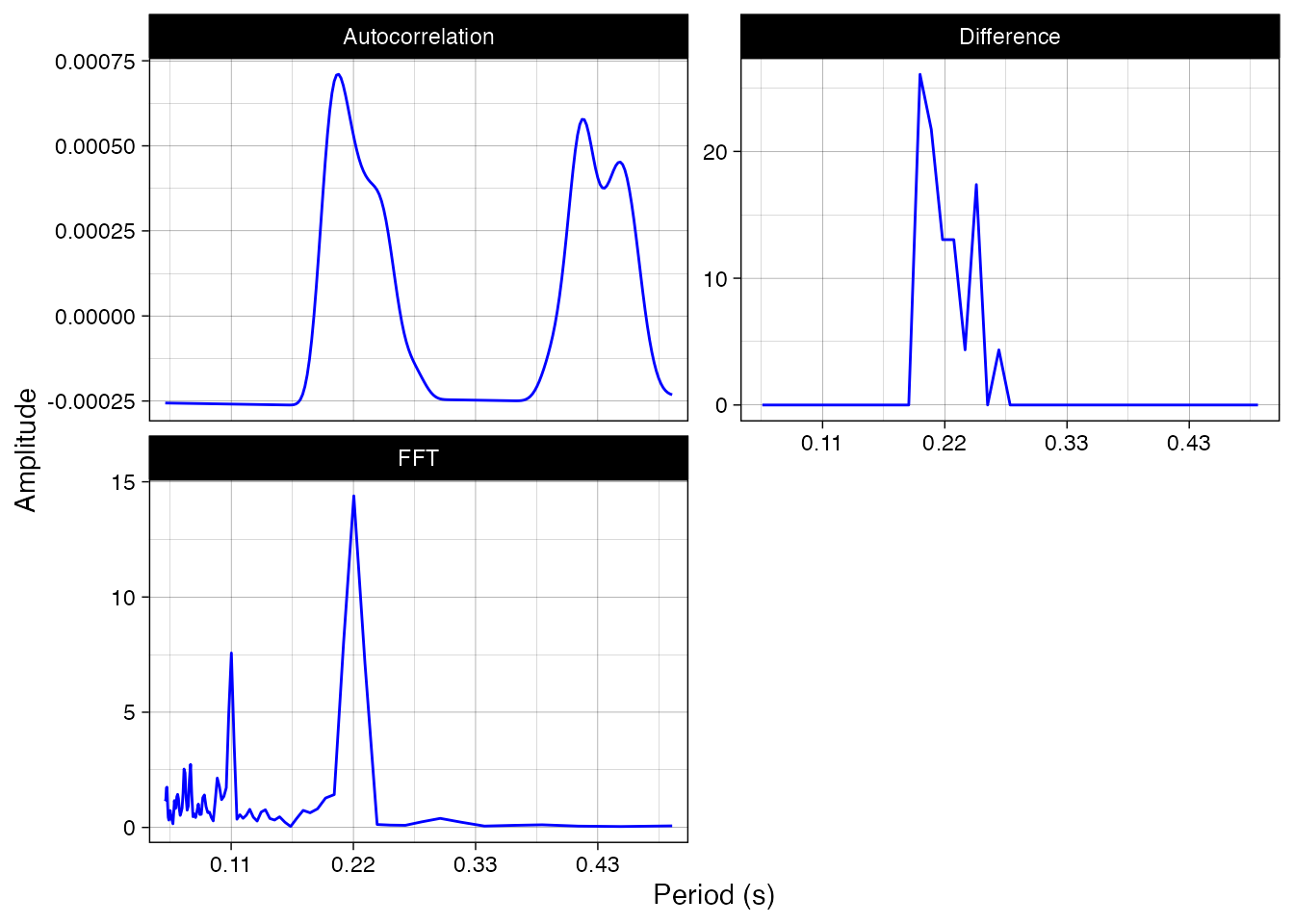
Figure 2. Periodicity analysis of a 5-second extract of guitar playing in Cuban son using difference in onset times as a primitive periodicity measure, the output from autocorrelation function, and the estimation of periodicity by FFT.
From the estimated periodicity curves, we can obtain the peak period in milliseconds, and if we so wish, we convert this into beats per minute (BPM). For the latter convention, we make use of the fact that the guitar plays four times per four beats.
PM <- summarise_periodicity(fig2D$Curve)
print(paste('Period of',round(PM$Per*1000),'ms'))
## [1] "Period of 217 ms"
print(paste(period_to_BPM(PM$Per)/4,'BPM'))## [1] "69 BPM"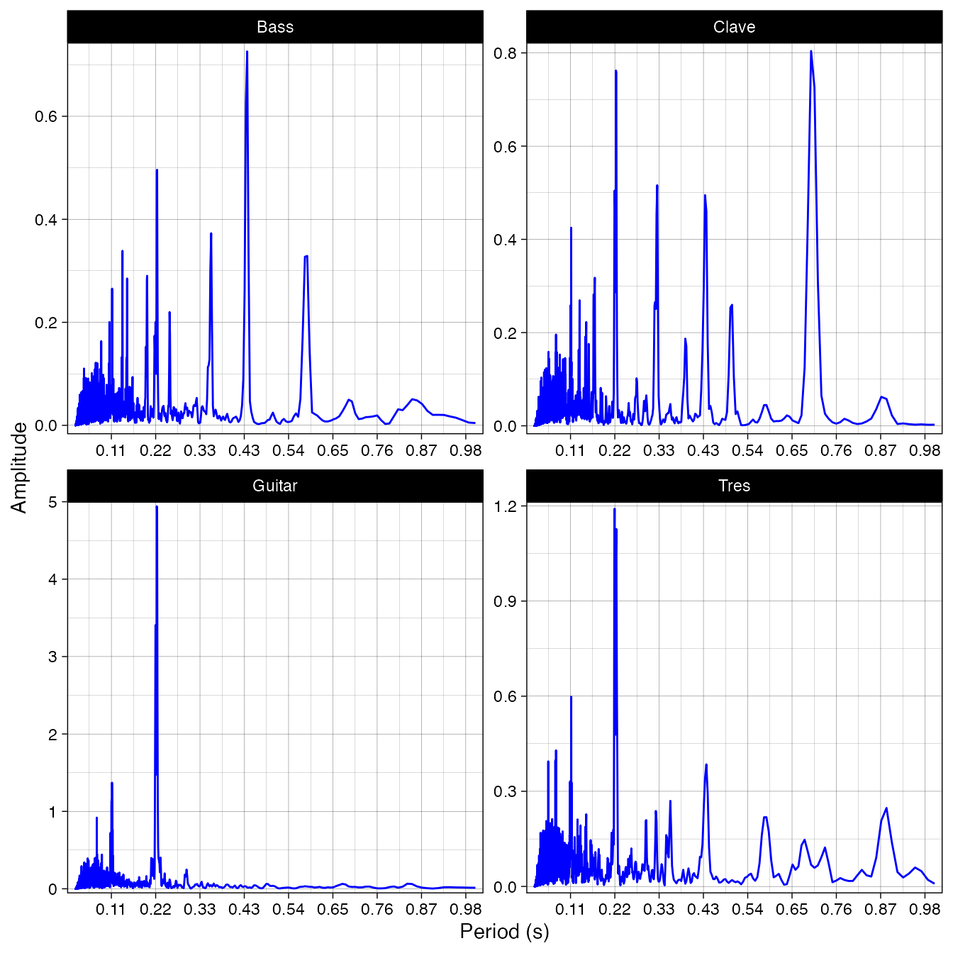
Figure 2. Periodicity analysis of four selected instruments in the example song (Palo Alto). The grid lines indicate multiples of the period identified earlier as the underlying beat (217 ms).
Being able to bring periodicity estimation of onset sequences into the analysis of asynchrony has many useful purposes. It can serve as a diagnostic into the periodic patterns performed by the instruments. This might be particularly useful if no annotation about the cycles and beat subdivisions is available and the analyst is trying to determine what are the periodicities exhibited by the different instruments. For instance, Figure 7 shows the periodicities of the selected four instruments in our salsa example. The analysis reveals that guitar and the tres tend to play the fastest beat pulsation (0.22 s) while the tres occasionally ventures into double (0.44 s) and four times the period (0.88 s). Bass shows three dominant periods, one at the fastest beat pulsation level (0.22), double of that period (0.44) and two uneven subdivisions of the underlying beat (0.35 s and 0.58 s). The clave’s pattern includes a period of 0.66 secs, three times the fastest pulse, presumably thanks to its pattern at the start of the cycle (when it plays on subdivisions 1, 4 & 7).