onsetsync is a R package for musical assessing synchrony between onsets in music. There are functions for common operations such as adding isochronous beats based on metrical structure, adding annotations, calculating classic measures of synchrony between performers, and assessing periodicity of the onsets, and visualising synchrony across cycles, time, or another property.
For documentation, see Quick Guide.
Installation
You can install the current version of onsetsync from Github by entering the following commands into R:
if (!require(devtools)) install.packages("devtools")
devtools::install_github("tuomaseerola/onsetsync", force = TRUE)
Usage
Reading in data
Read onsets of one Cuban Son performance titled Palo Santo from IEMP dataset at https://osf.io/sfxa2/. This song has the onsets and the annotations about the metric cycles already extracted and defined and comes with the package.
Go and listen to the song at OSF.
CSS_Song2 <- onsetsync::CSS_IEMP[[2]]  # Read one song from internal data
CSS_Song2 <- dplyr::select(CSS_Song2,Label.SD,SD,Clave,Bass,Guitar,Tres,
                           CycleTime,Cycle,Isochronous.SD.Time) # Select some columns
print(knitr::kable(head(CSS_Song2),format = "simple",digits = 2))| Label.SD | SD | Clave | Bass | Guitar | Tres | CycleTime | Cycle | Isochronous.SD.Time |
|---|---|---|---|---|---|---|---|---|
| 1:1 | 1 | NA | NA | NA | NA | 5.04 | 1 | 5.04 |
| 1:2 | 2 | NA | NA | 5.28 | NA | NA | 1 | 5.26 |
| 1:3 | 3 | NA | NA | 5.48 | NA | NA | 1 | 5.48 |
| 1:4 | 4 | NA | 5.71 | 5.71 | 5.73 | NA | 1 | 5.71 |
| 1:5 | 5 | NA | 5.93 | 5.94 | 5.92 | NA | 1 | 5.93 |
| 1:6 | 6 | NA | NA | 6.15 | 6.14 | NA | 1 | 6.15 |
Reading data from is easy either from CSV files in your computer or directly from OSF using get_OSF_csv function.
Visualise onsets structures
As an overview, we can visualise the onsets across the beat sub-divisions for each instrument and do this across the time. Note that time run vertically (from bottom to up) here.
fig1 <- plot_by_beat(df = CSS_Song2,
                     instr = c('Bass','Clave','Guitar','Tres'),
                     beat = 'SD',
                     virtual='Isochronous.SD.Time',
                     pcols=2)
print(fig1)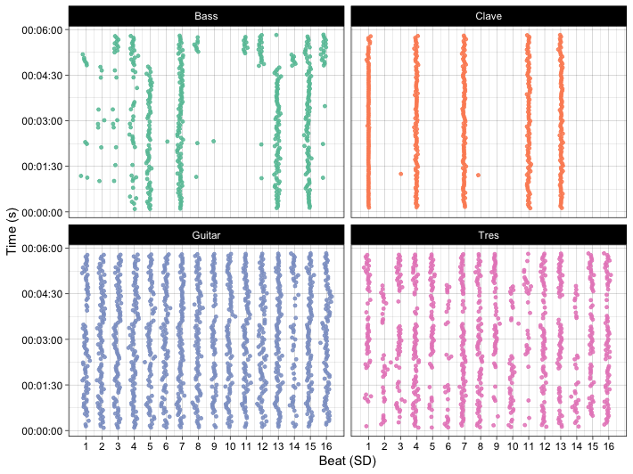
Calculate asynchronies
To what degree are the pairs of instruments synchronised to each other? Let’s visualise the synchrony of all pairings of the instruments in this example.
inst <- c('Clave','Bass','Guitar','Tres')              # Define instruments
dn <- sync_execute_pairs(CSS_Song2, inst, beat = 'SD') # Calculate ansychr.
fig2 <- plot_by_pair(dn)                               # Plot
print(fig2) 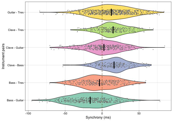
As we saw in the first figure, the instruments usually play widely different amounts of onsets in a piece, and these are bound to be at different beats sub-divisions, the mutual amount of comparable onsets for each pair often varies dramatically. Comparison of mean asynchronies across sub-divisions can be facilitated by taking random samples of the joint onsets. Here we choose a random 200 matching onsets and re-calculate the comparison of asynchrony with this subset 1000 times.
set.seed(1234) # set random seed
N <- 200 # Let's select 200 onsets
Bootstrap <- 100 # Let's bootstrap this 100 times
d1 <- sync_sample_paired(df=CSS_Song2,
                         instr1 = 'Clave',
                         instr2 = 'Bass',
                         n = N,
                         bootn = Bootstrap,
                         beat = 'SD')
dplyr::summarise(data.frame(d1), N=n(), M = mean(asynch*1000), SD = sd(asynch*1000))
#>       N        M       SD
#> 1 20000 16.26593 19.54912
There are other measures to summarise the asynchronies and visualise them.
For more examples, see Get started.