Exp. 2 - Higher Order Structures

Load data

df_f <- readRDS("data/items35_N1200.rds")
source('scr/rename_specific_items.R') # We decided to relabel some constructs for clarity
df_f <- rename_specific_items(df_f)
# F1 should be in Motivation, relabelled as M9
df_f$item_label[df_f$item_label=="F1"] <- "M9"

source('scr/CFA_items.R')

Higher order structures

These analysyses correspond to section Reliability, discriminant validity and convergent validity of the scales in the manuscript.

First-Order Model (sub-constructs)

Let’s explore how the episodes operate via 12 sub-constructs.

set.seed(3110)

first_order <- "
# sub-factors: EDR
E =~ E1 + E6 + E7
D =~ D1 + D6 + D7
R =~ R1 + R3 + R7

# sub-factors: FM
M =~ M1 + M3 + M9
F =~ F3 + F6 + F10

# sub-factors: CB
G =~ G5 + G2 + G9
L =~ L5 + L6 + L7

# sub-factors: PEP
C =~ C2 + C3 + C6
X =~ X4 + X8 + X9

# sub-factors: AIA
S =~ S3 + S4 + S5
I =~ I1 + I2
B =~ B1 + B3 + B5
"

items <- c("E1","E6","E7","D1","D6","D7","R1","R3","R7","M1","M3","M9","F3","F6","F10","G5","G2","G9","L5","L6","L7","C2","C3","C6","X4","X8","X9","S3","S4","S5","I1","I2","B1","B3","B5")
tmp <- CFA_items(df_f,vignette = 1:12, items=items,vignette_name="ALL",bonusquestion="HAAS")
fit1 <- lavaan::cfa(model = first_order, data = tmp, meanstructure = TRUE,estimator = "MLR")
fit1.meas <- lavaan::fitMeasures(fit1,c("tli","chisq","df","pvalue", "cfi", "rmsea", "srmr"))
print(fit1.meas)

     tli    chisq       df   pvalue      cfi    rmsea     srmr 
   0.949 1617.750  494.000    0.000    0.958    0.044    0.039

First and Second-Order Model

Let’s explore how the episodes (Constructs) operate when build as second-order model with sub-constructs.

set.seed(3110)

second_order <- "
# sub-factors: EDR
E =~ E1 + E6 + E7
D =~ D1 + D6 + D7
R =~ R1 + R3 + R7

# sub-factors: FM
M =~ M1 + M3 + M9
F =~ F3 + F6 + F10

# sub-factors: CB
G =~ G5 + G2 + G9
L =~ L5 + L6 + L7

# sub-factors: PEP
C =~ C2 + C3 + C6
X =~ X4 + X8 + X9

# sub-factors: AIA
S =~ S3 + S4 + S5
I =~ I1 + I2
B =~ B1 + B3 + B5

# 2nd order factors

EDR =~ E + D + R
FM =~ M + F
CB =~ G + L 
PEP =~ C + X
AIA =~ S + I + B  
"

items <- c("E1","E6","E7","D1","D6","D7","R1","R3","R7","M1","M3","M9","F3","F6","F10","G5","G2","G9","L5","L6","L7","C2","C3","C6","X4","X8","X9","S3","S4","S5","I1","I2","B1","B3","B5")

tmp <- CFA_items(df_f,vignette = 1:12, items=items,vignette_name="ALL",bonusquestion="HAAS")
fit2 <- lavaan::cfa(model = second_order, data = tmp, meanstructure = TRUE, estimator = "MLR")

Warning: lavaan->lav_object_post_check():  
   covariance matrix of latent variables is not positive definite ; use 
   lavInspect(fit, "cov.lv") to investigate.

fit2.meas <- lavaan::fitMeasures(fit2,c("tli","chisq","df","pvalue", "cfi", "rmsea", "srmr"))
print(fit2.meas)

     tli    chisq       df   pvalue      cfi    rmsea     srmr 
   0.918 2512.255  538.000    0.000    0.926    0.055    0.060

Bi-factor Model

Test whether the items load on both a general factor and their specific episode factors (sub-constructs).

Warning: lavaan->lav_model_vcov():  
   The variance-covariance matrix of the estimated parameters (vcov) does not 
   appear to be positive definite! The smallest eigenvalue (= -9.586897e-06) 
   is smaller than zero. This may be a symptom that the model is not 
   identified.

     tli    chisq       df   pvalue      cfi    rmsea     srmr 
   0.901 2854.587  525.000    0.000    0.913    0.061    0.065

Second-order Model only

Test whether the items work through 5 constructs only (all sub-constructs are included in each construct).

     tli    chisq       df   pvalue      cfi    rmsea     srmr 
   0.678 8516.714  550.000    0.000    0.702    0.110    0.100

First-order, Second-order and a Generic Third-order

Warning: lavaan->lav_object_post_check():  
   some estimated lv variances are negative

     tli    chisq       df   pvalue      cfi    rmsea     srmr 
   0.917 2561.692  543.000    0.000    0.925    0.056    0.062

Visualise Models

First-order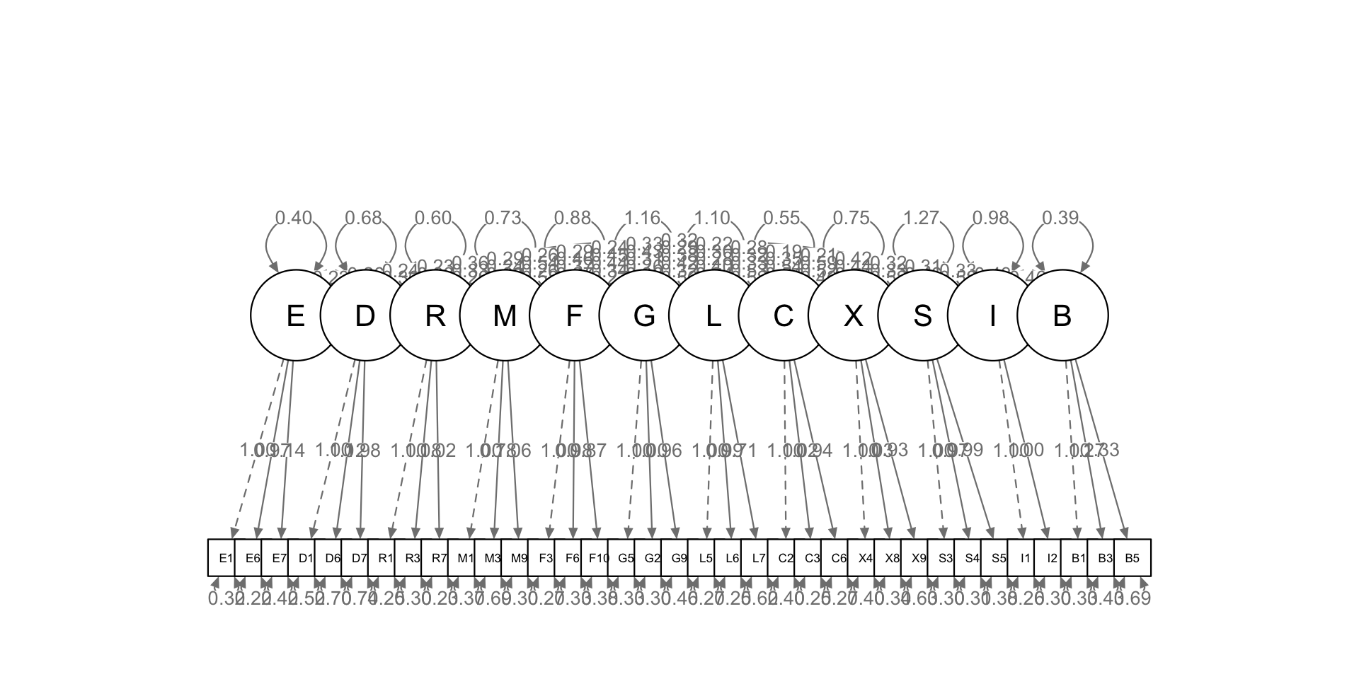

First and second-order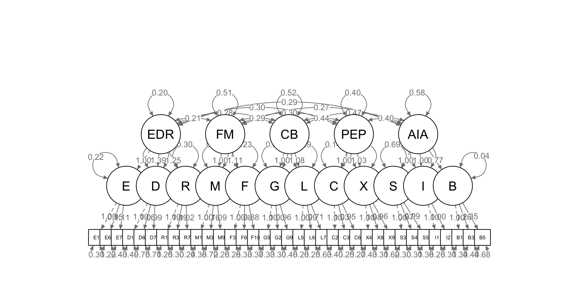

Bifactor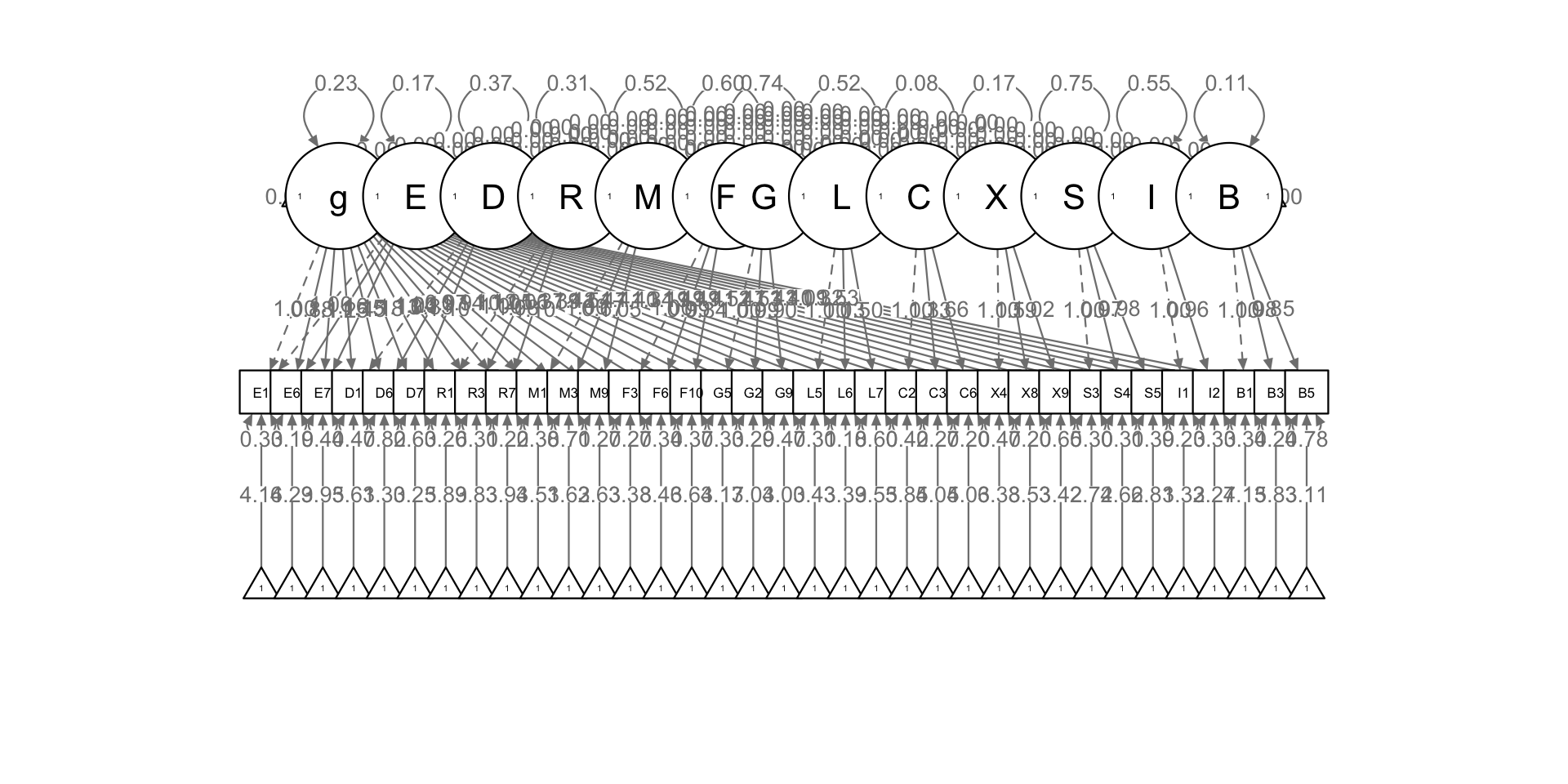

Second-order only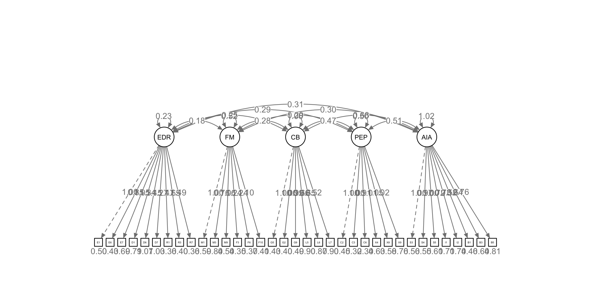

1st, 2nd, and third-order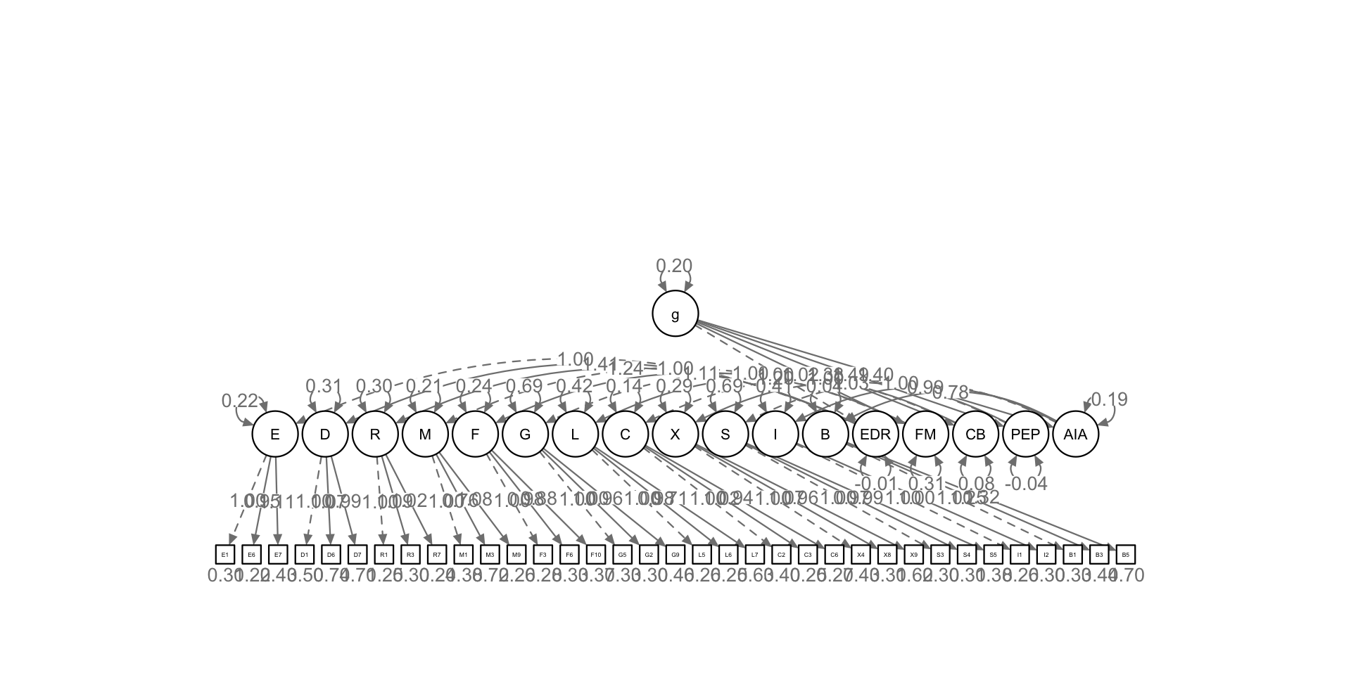

Summarise Model Fits

	tli	chisq	df	cfi	rmsea	srmr
1st-order	0.95	1617.75	494	0.96	0.04	0.04
1st and 2nd-order	0.92	2512.25	538	0.93	0.06	0.06
Bifactor	0.90	2854.59	525	0.91	0.06	0.07
Second-order only	0.68	8516.71	550	0.70	0.11	0.10
1-,2-, 3rd-order	0.92	2561.69	543	0.92	0.06	0.06

Compare Structures

In the manuscript, we only report first-order and second-order models, as the other candidates are significantly worse (conceptually and statistically).

o <- compareFit(fit1, fit2)
summary(o)

################### Nested Model Comparison #########################

Scaled Chi-Squared Difference Test (method = "satorra.bentler.2001")

lavaan->unknown():  
   lavaan NOTE: The "Chisq" column contains standard test statistics, not the 
   robust test that should be reported per model. A robust difference test is 
   a function of two standard (not robust) statistics.
      Df   AIC    BIC  Chisq Chisq diff Df diff Pr(>Chisq)    
fit1 494 98873  99743 1617.8                                  
fit2 538 99679 100326 2512.3     689.07      44  < 2.2e-16 ***
---
Signif. codes:  0 '***' 0.001 '**' 0.01 '*' 0.05 '.' 0.1 ' ' 1

####################### Model Fit Indices ###########################
     chisq.scaled df.scaled pvalue.scaled rmsea.robust cfi.robust tli.robust
fit1    1362.501†       494          .000        .042†      .961†      .953†
fit2    2099.846        538          .000        .054       .930       .922 
      srmr        aic         bic
fit1 .039† 98872.698†  99743.101†
fit2 .060  99679.203  100325.643 

################## Differences in Fit Indices #######################
            df.scaled rmsea.robust cfi.robust tli.robust  srmr     aic     bic
fit2 - fit1        44        0.012     -0.031     -0.031 0.021 806.505 582.541

Construct Reliability (Composite Reliability)

Measure of internal consistency using omega from the second-order model.

# Calculate reliability indices:
# 0.60 questionable, 0.70 acceptable, 0.80 good, 0.90 excellent
# This is done using omega, not alpha
compRelSEM(fit1,tau.eq=F)                 # all acceptable good excellent

    E     D     R     M     F     G     L     C     X     S     I     B 
0.806 0.769 0.882 0.818 0.878 0.903 0.881 0.842 0.829 0.918 0.874 0.783

compRelSEM(fit2,higher = c("EDR","FM","CB","PEP","AIA"),tau.eq=F) # all acceptable good excellent

    E     D     R     M     F     G     L     C     X     S     I     B   EDR 
0.804 0.771 0.882 0.811 0.879 0.903 0.880 0.841 0.832 0.918 0.874 0.783 0.679 
   FM    CB   PEP   AIA 
0.760 0.613 0.704 0.759

compRelSEM(fit3, tau.eq=F)               # g good but constructs are poor

    g     E     D     R     M     F     G     L     C     X     S     I     B 
0.894 0.386 0.373 0.470 0.531 0.588 0.551 0.394 0.234 0.285 0.539 0.472 0.250

compRelSEM(fit4,tau.eq=F)                # all above 0.80

  EDR    FM    CB   PEP   AIA 
0.836 0.864 0.833 0.844 0.886

compRelSEM(fit5,tau.eq=F,higher="g")     # all above 0.80

    E     D     R     M     F     G     L     C     X     S     I     B     g 
0.805 0.771 0.882 0.812 0.879 0.903 0.880 0.842 0.832 0.918 0.874 0.782   NaN

cor_matrix <- lavInspect(fit2, "cor.lv")
print(knitr::kable(cor_matrix,digits=2,caption="Correlations between the latent factors (for sub-constructs and constructs)."))



Table: Correlations between the latent factors (for sub-constructs and constructs).

|    |    E|    D|    R|    M|    F|    G|    L|    C|    X|    S|    I|    B|  EDR|   FM|   CB|  PEP|  AIA|
|:---|----:|----:|----:|----:|----:|----:|----:|----:|----:|----:|----:|----:|----:|----:|----:|----:|----:|
|E   | 1.00| 0.51| 0.49| 0.39| 0.39| 0.40| 0.44| 0.64| 0.57| 0.40| 0.45| 0.56| 0.69| 0.46| 0.59| 0.74| 0.59|
|D   | 0.51| 1.00| 0.52| 0.41| 0.42| 0.43| 0.47| 0.68| 0.61| 0.42| 0.48| 0.59| 0.73| 0.49| 0.63| 0.79| 0.62|
|R   | 0.49| 0.52| 1.00| 0.40| 0.40| 0.41| 0.46| 0.66| 0.59| 0.41| 0.47| 0.57| 0.71| 0.47| 0.61| 0.76| 0.61|
|M   | 0.39| 0.41| 0.40| 1.00| 0.72| 0.32| 0.35| 0.49| 0.44| 0.28| 0.32| 0.39| 0.56| 0.84| 0.47| 0.57| 0.41|
|F   | 0.39| 0.42| 0.40| 0.72| 1.00| 0.32| 0.36| 0.49| 0.44| 0.28| 0.32| 0.40| 0.57| 0.85| 0.48| 0.57| 0.42|
|G   | 0.40| 0.43| 0.41| 0.32| 0.32| 1.00| 0.50| 0.56| 0.51| 0.38| 0.44| 0.54| 0.58| 0.38| 0.67| 0.65| 0.57|
|L   | 0.44| 0.47| 0.46| 0.35| 0.36| 0.50| 1.00| 0.62| 0.56| 0.43| 0.48| 0.60| 0.64| 0.42| 0.74| 0.72| 0.63|
|C   | 0.64| 0.68| 0.66| 0.49| 0.49| 0.56| 0.62| 1.00| 0.67| 0.48| 0.55| 0.68| 0.92| 0.58| 0.83| 0.86| 0.72|
|X   | 0.57| 0.61| 0.59| 0.44| 0.44| 0.51| 0.56| 0.67| 1.00| 0.44| 0.49| 0.61| 0.83| 0.52| 0.75| 0.77| 0.64|
|S   | 0.40| 0.42| 0.41| 0.28| 0.28| 0.38| 0.43| 0.48| 0.44| 1.00| 0.52| 0.64| 0.58| 0.33| 0.57| 0.56| 0.68|
|I   | 0.45| 0.48| 0.47| 0.32| 0.32| 0.44| 0.48| 0.55| 0.49| 0.52| 1.00| 0.73| 0.65| 0.38| 0.65| 0.64| 0.77|
|B   | 0.56| 0.59| 0.57| 0.39| 0.40| 0.54| 0.60| 0.68| 0.61| 0.64| 0.73| 1.00| 0.81| 0.46| 0.80| 0.79| 0.95|
|EDR | 0.69| 0.73| 0.71| 0.56| 0.57| 0.58| 0.64| 0.92| 0.83| 0.58| 0.65| 0.81| 1.00| 0.66| 0.86| 1.07| 0.85|
|FM  | 0.46| 0.49| 0.47| 0.84| 0.85| 0.38| 0.42| 0.58| 0.52| 0.33| 0.38| 0.46| 0.66| 1.00| 0.56| 0.67| 0.49|
|CB  | 0.59| 0.63| 0.61| 0.47| 0.48| 0.67| 0.74| 0.83| 0.75| 0.57| 0.65| 0.80| 0.86| 0.56| 1.00| 0.97| 0.84|
|PEP | 0.74| 0.79| 0.76| 0.57| 0.57| 0.65| 0.72| 0.86| 0.77| 0.56| 0.64| 0.79| 1.07| 0.67| 0.97| 1.00| 0.83|
|AIA | 0.59| 0.62| 0.61| 0.41| 0.42| 0.57| 0.63| 0.72| 0.64| 0.68| 0.77| 0.95| 0.85| 0.49| 0.84| 0.83| 1.00|

Discriminant Validity

Average Variance Explained (traditional)

Measure of discriminant validity from the first-order model.

# calculate average variance explained, 0.50+ is acceptable 
lavInspect(fit1, "cor.lv")

      E     D     R     M     F     G     L     C     X     S     I     B
E 1.000                                                                  
D 0.432 1.000                                                            
R 0.518 0.555 1.000                                                      
M 0.449 0.467 0.300 1.000                                                
F 0.381 0.429 0.409 0.724 1.000                                          
G 0.521 0.271 0.306 0.298 0.270 1.000                                    
L 0.432 0.623 0.450 0.381 0.390 0.502 1.000                              
C 0.559 0.747 0.760 0.410 0.462 0.431 0.668 1.000                        
X 0.535 0.635 0.467 0.565 0.491 0.574 0.595 0.667 1.000                  
S 0.337 0.459 0.428 0.295 0.313 0.445 0.438 0.524 0.531 1.000            
I 0.529 0.361 0.389 0.374 0.375 0.553 0.429 0.454 0.533 0.517 1.000      
B 0.807 0.428 0.579 0.353 0.357 0.620 0.484 0.678 0.608 0.612 0.748 1.000

# First-order model
AVE(fit1)  # all above 0.50

    E     D     R     M     F     G     L     C     X     S     I     B 
0.579 0.528 0.713 0.596 0.708 0.756 0.704 0.636 0.615 0.789 0.776 0.541

# First and second-order
AVE(fit2)  # all above 0.50

    E     D     R     M     F     G     L     C     X     S     I     B 
0.577 0.528 0.713 0.594 0.708 0.756 0.704 0.635 0.617 0.789 0.776 0.541

# Bifactor
AVE(fit3,omit.factors="g")  # All below 0.50

    E     D     R     M     F     G     L     C     X     S     I     B 
0.277 0.259 0.380 0.394 0.475 0.462 0.339 0.184 0.222 0.464 0.420 0.196

# Second-order only
AVE(fit4)  # FM, CB and AIA above 0.50, EDR and PEP below 0.50

  EDR    FM    CB   PEP   AIA 
0.383 0.539 0.520 0.493 0.513

# 1st, 2nd, and third-order
AVE(fit5)  # all above 0.50

    E     D     R     M     F     G     L     C     X     S     I     B 
0.577 0.529 0.713 0.594 0.708 0.756 0.704 0.636 0.617 0.789 0.776 0.540

Discriminant Validity with HTMT

Let’s use the modern Heterotrait–Monotrait Ratio (HTMT) method to assess discriminant validity. It uses ratio of the correlations (Henseler, Ringlet & Sarstedt, 2015).

All Sub-constructs (first-order model)

htmt_matrix <- htmt(first_order,data = tmp,htmt2 = FALSE)
print(knitr::kable(htmt_matrix,digits=3,caption='Discriminant Validity at the level of Sub-Constructs.'))

Discriminant Validity at the level of Sub-Constructs.
	E	D	R	M	F	G	L	C	X	S	I	B
E	1.000	0.443	0.521	0.515	0.396	0.525	0.463	0.563	0.542	0.338	0.528	0.809
D	0.443	1.000	0.552	0.459	0.426	0.276	0.654	0.745	0.654	0.458	0.358	0.431
R	0.521	0.552	1.000	0.272	0.405	0.309	0.494	0.760	0.474	0.429	0.388	0.577
M	0.515	0.459	0.272	1.000	0.721	0.346	0.424	0.401	0.597	0.299	0.405	0.394
F	0.396	0.426	0.405	0.721	1.000	0.280	0.444	0.464	0.497	0.315	0.379	0.367
G	0.525	0.276	0.309	0.346	0.280	1.000	0.514	0.432	0.568	0.451	0.552	0.633
L	0.463	0.654	0.494	0.424	0.444	0.514	1.000	0.714	0.631	0.472	0.460	0.517
C	0.563	0.745	0.760	0.401	0.464	0.432	0.714	1.000	0.682	0.534	0.459	0.688
X	0.542	0.654	0.474	0.597	0.497	0.568	0.631	0.682	1.000	0.532	0.536	0.619
S	0.338	0.458	0.429	0.299	0.315	0.451	0.472	0.534	0.532	1.000	0.517	0.618
I	0.528	0.358	0.388	0.405	0.379	0.552	0.460	0.459	0.536	0.517	1.000	0.758
B	0.809	0.431	0.577	0.394	0.367	0.633	0.517	0.688	0.619	0.618	0.758	1.000

diag(htmt_matrix)=NA
round(min(htmt_matrix,na.rm=TRUE),3)

[1] 0.272

round(max(htmt_matrix,na.rm=TRUE),3)

[1] 0.809

round(median(htmt_matrix,na.rm=TRUE),3)

[1] 0.484

All Constructs (second-order model)

htmt_matrix <- htmt(episodes,data = tmp,htmt2 = FALSE)
print(knitr::kable(htmt_matrix,digits=3,caption='Discriminant Validity at the level of Constructs.'))

Discriminant Validity at the level of Constructs.
	EDR	FM	CB	PEP	AIA
EDR	1.000	0.565	0.672	0.871	0.712
FM	0.565	1.000	0.484	0.596	0.459
CB	0.672	0.484	1.000	0.771	0.719
PEP	0.871	0.596	0.771	1.000	0.740
AIA	0.712	0.459	0.719	0.740	1.000

diag(htmt_matrix)=NA
round(min(htmt_matrix,na.rm=TRUE),3)

[1] 0.459

round(max(htmt_matrix,na.rm=TRUE),3)

[1] 0.871

round(median(htmt_matrix,na.rm=TRUE),3)

[1] 0.692