Exp. 1 - Preprocessing

Load and preprocess data

source('scr/read_EFA_qualtrics.R') # custom function
fn <- "data/EDR - Pilot_August 18, 2025_10.15.csv"
d1 <- read_EFA_qualtrics(filename = fn, subconstructs = c("E","D","R"))

[1] "data/EDR - Pilot_August 18, 2025_10.15.csv"
[1] "E" "D" "R"
NULL
[1] "Number of participants in the data: 120"
[1] "Number of participants after filter incomplete/preview/99 age: 106"
[1] "Inattentive in total: 0"
[1] "The IDs of the inattentive participants are:"
character(0)
[1] "Number of accepted participants: 106"

df1<- convert_items_long(d1)

[1] "EDR items loaded"

df1b<- participant_reliability(df1,THRESHOLD = 0.001)

[1] "Alpha: 0.97"
[1] "Eliminate the worst participants (r below THRESHOLD)"
[1] "Number of participants to eliminate: 6"
[1] "6813ef0e8fdad3ca067b605e" "6772fe0fba57bc97da6950a5"
[3] "6659f6fdd8cd7577c303a76d" "5c7ed8dfe82bf100010fb514"
[5] "62fbe4c86d484357b6adbc36" "67d411652ada0a7584b2558e"
[1] "Alpha: 0.97"
[1] "N after trimming: 100"

df1b$study <- 1

fn <- "data/FM_August 27, 2025_04.04.csv"
d2 <- read_EFA_qualtrics(filename=fn,subconstructs = c("F","M"), controlQ = "M_15")

[1] "data/FM_August 27, 2025_04.04.csv"
[1] "F" "M"
[1] "M_15"
[1] "Number of participants in the data: 109"
[1] "Number of participants after filter incomplete/preview/99 age: 107"
[1] "Inattentive in total: 4"
[1] "The IDs of the inattentive participants are:"
[1] "65537e14439274fe5036b4d2" "66c605bf16b21d64057a018b"
[3] "5de3c83c2033793be6591e53" "6658c56f3d9230d99c3e6752"
[1] "Number of accepted participants: 103"

df2<- convert_items_long(d2)

[1] "FM items loaded"

df2b<- participant_reliability(df2,THRESHOLD = 0.001)

[1] "Alpha: 0.98"
[1] "Eliminate the worst participants (r below THRESHOLD)"
[1] "Number of participants to eliminate: 3"
[1] "67e19f44ba489abd4e850452" "5f27f6a0e13d4e05d048335f"
[3] "66a50183d6f19b4257015e67"
[1] "Alpha: 0.99"
[1] "N after trimming: 100"

df2b$study <- 2

fn <- "data/CB - redo_September 1, 2025_03.36.csv"
d3 <- read_EFA_qualtrics(filename=fn,subconstructs = c("C","S"), controlQ = "C_16")

[1] "data/CB - redo_September 1, 2025_03.36.csv"
[1] "C" "S"
[1] "C_16"
[1] "Number of participants in the data: 120"
[1] "Number of participants after filter incomplete/preview/99 age: 116"
[1] "Inattentive in total: 4"
[1] "The IDs of the inattentive participants are:"
[1] "654f89d4924d0d5a050f375d" "67129f965260be663a982f67"
[3] "5eab170759f5390b776df5a1" "666ee5994b49ad9236867a62"
[1] "Number of accepted participants: 112"

df3<- convert_items_long(d3)

[1] "CB items loaded"

df3b<- participant_reliability(df3,THRESHOLD = 0.001)

[1] "Alpha: 0.95"
[1] "Eliminate the worst participants (r below THRESHOLD)"
[1] "Number of participants to eliminate: 12"
 [1] "5be4c588854f100001537d04" "6070eac7c04a391b5267809f"
 [3] "5f4a9eb861da210d3496cb34" "5fe7bc4ec39215684de426f4"
 [5] "6012d27152fa5e09eb6a29e0" "672946ef8187e4253c5ff800"
 [7] "5ab87be55cd105000161a5a8" "645e967fad9bc8bdc1a16ac0"
 [9] "5ef20e5fa9ac1301228a263a" "5a53991eac56240001537454"
[11] "5cb4f4ec46ed130001d15b05" "66b1375b72c3a0f57828dcca"
[1] "Alpha: 0.96"
[1] "N after trimming: 100"

df3b$study <- 3

fn <- "data/PEP_September 2, 2025_07.17.csv"
d4 <- read_EFA_qualtrics(filename=fn,subconstructs = c("U","P"), controlQ = "U_21")

[1] "data/PEP_September 2, 2025_07.17.csv"
[1] "U" "P"
[1] "U_21"
[1] "Number of participants in the data: 125"
[1] "Number of participants after filter incomplete/preview/99 age: 123"
[1] "Inattentive in total: 16"
[1] "The IDs of the inattentive participants are:"
 [1] "5d8878251f684d0001737c56" "67c83488e67b25dcb923d96d"
 [3] "6659fdbefa66c9fbb5cfcdf9" "5c26ac6163e1d8000103824f"
 [5] "5f0f6811a0ed4a11dbc57b79" "61364d250433ee40764f71b4"
 [7] "5e204990b062543612e9a254" "60b3950b9a1de417d37bb8d2"
 [9] "6071933c3c4ea940e3e2f175" "5a2c51740a1e6b00016952c8"
[11] "56f52b95298124000a8ef248" "5e46ff334267181cd82562e0"
[13] "612399c71548ff3b47e406e8" "5ea1d789f5c6d70c14fbe739"
[15] "6712264b956f8f9b305ee14b" "641571922d04f807e7157a04"
[1] "Number of accepted participants: 107"

df4<- convert_items_long(d4)

[1] "PEP items loaded"

df4b<- participant_reliability(df4,THRESHOLD = 0.001)

[1] "Alpha: 0.93"
[1] "Eliminate the worst participants (r below THRESHOLD)"
[1] "Number of participants to eliminate: 7"
[1] "65fb70d4e69155a62d58ac90" "61fa9112d42cb19beec492b5"
[3] "6765e84a9352323bd525b324" "612d4269137ff0bcf765ba63"
[5] "58404fd8ad98e40001ce915f" "6109ab5c911c8036b524515c"
[7] "5e15047894d5eeb157532e7f"
[1] "Alpha: 0.94"
[1] "N after trimming: 100"

df4b$study <- 4

fn <- "data/AIA_September 3, 2025_05.02.csv"
d5 <- read_EFA_qualtrics(filename=fn,subconstructs = c("I","X","B"), controlQ = "I_17")

[1] "data/AIA_September 3, 2025_05.02.csv"
[1] "I" "X" "B"
[1] "I_17"
[1] "Number of participants in the data: 113"
[1] "Number of participants after filter incomplete/preview/99 age: 111"
[1] "Inattentive in total: 9"
[1] "The IDs of the inattentive participants are:"
[1] "6130a2a2e00bc5b94c8b83e7" "5ee50501a3c8f8235ea18d0e"
[3] "5eeb4ad567a40221fd8a1a04" "572f8258ad13160010008a61"
[5] "65b3d516eaf68da25cef67d6" "61446a1ecda939d3c22d9787"
[7] "602ba5af8055272f9a36e3fe" "5e64f63fe8177d2669776c08"
[9] "6426cfe964863ee2ff26642f"
[1] "Number of accepted participants: 102"

df5<- convert_items_long(d5)

[1] "AIA items loaded"

df5b<- participant_reliability(df5,THRESHOLD = 0.001)

[1] "Alpha: 0.98"
[1] "Eliminate the worst participants (r below THRESHOLD)"
[1] "Number of participants to eliminate: 1"
[1] "66f0765bb7f6c2ae6ef721ee"
[1] "Alpha: 0.98"
[1] "N after trimming: 101"

df5b$study <- 5

Demographics

Setting up demographic analysis.

demographics <- rbind(df1b, df2b, df3b, df4b, df5b)
demo_clean <- demographics[!duplicated(demographics$ID),]

#aov.age <- aov(demo_clean$study ~ demo_clean$Age, data = demo_clean) # this is wrong
aov.age <- aov(Age ~ factor(study), data = demo_clean) # this is correct
summary(aov.age)

               Df Sum Sq Mean Sq F value Pr(>F)
factor(study)   4   1020   255.0   1.533  0.191
Residuals     496  82493   166.3               

demo_clean<-dplyr::filter(demo_clean,Gender!="Non-binary")
ch.gender <- chisq.test(demo_clean$Gender, factor(demo_clean$study),simulate.p.value = FALSE)
print(knitr::kable(table(demo_clean$Gender, demo_clean$study))) 

|       |  1|  2|  3|  4|  5|
|:------|--:|--:|--:|--:|--:|
|Female | 41| 55| 50| 69| 58|
|Male   | 58| 45| 50| 31| 43|

ch.gender

    Pearson's Chi-squared test

data:  demo_clean$Gender and factor(demo_clean$study)
X-squared = 16.495, df = 4, p-value = 0.002423

M <- as.table(rbind(c(69, 31), c(50, 50))) # extreme group
print(chisq.test(M))

    Pearson's Chi-squared test with Yates' continuity correction

data:  M
X-squared = 6.7227, df = 1, p-value = 0.009519

M <- as.table(rbind(c(41, 58), c(50, 50)))
chisq.test(M)

    Pearson's Chi-squared test with Yates' continuity correction

data:  M
X-squared = 1.152, df = 1, p-value = 0.2831

table(demo_clean$OMSI)

         Amateur musician  Music-loving Nonmusician               Nonmusician 
                       66                       320                        89 
    Professional musician Semiprofessional musician  Serious amateur musician 
                        3                         7                        15 

ch.OMSI <- chisq.test(demo_clean$OMSI, factor(demo_clean$study),simulate.p.value = FALSE) # Correct

Warning in chisq.test(demo_clean$OMSI, factor(demo_clean$study),
simulate.p.value = FALSE): Chi-squared approximation may be incorrect

ch.OMSI

    Pearson's Chi-squared test

data:  demo_clean$OMSI and factor(demo_clean$study)
X-squared = 24.753, df = 20, p-value = 0.211

table(demo_clean$OMSI,demo_clean$study)

                           
                             1  2  3  4  5
  Amateur musician          13  5 11 17 20
  Music-loving Nonmusician  66 72 61 61 60
  Nonmusician               16 20 23 14 16
  Professional musician      1  0  2  0  0
  Semiprofessional musician  1  1  1  2  2
  Serious amateur musician   2  2  2  6  3

#aov.OMSI <- aov(demo_clean$study ~ demo_clean$OMSI, data = demo_clean)

#OMSI <- c("Nonmusician" = 1, "Music-loving Nonmusician" = 2, "Amateur musician" = 3, "Serious amateur musician" = 4, "Semiprofessional musician" = 5, "Professional musician" = 5)

#table(demo_clean$Gender)
#Gender <- c("Female" = 1, "Male" = 2, "Non-binary" = 3, "Other" = 4, "Prefer not to say" = 5)

Looking at Relevance

EDRrel <- c(d1$D_Rep, d1$R_Rel, d1$E_Rel)
FMrel <- c(d2$M_Rel, d2$F_Rel)
CBrel <- c(d3$S_Rel, d3$C_Rel)
PEPrel <- c(d4$P_Rel, d4$U_Rel)
AIArel <- c(d5$B_Rel, d5$X_Rel, d5$I_Rel)

Save preprocessed data

Before running any structural analysis, let’s revise the item names.

save_requested <- FALSE
if(save_requested==TRUE){
  saveRDS(df1b,file="data/EDR_N100.rds")
  saveRDS(df2b,file="data/FM_N100.rds")
  saveRDS(df3b,file="data/CB_N100.rds")
  saveRDS(df4b,file="data/PEP_N100.rds")
  saveRDS(df5b,file="data/AIA_N101.rds")
}

Looking at various reliability estimates

From Revelle & Condon, 2019; Shrout & Lane, 2012. See Vispoel, Morris, & Kilinc, 2018; ten Hove, Jorgensen, & van der Ark, 2022

source('scr/ml_r.R') #just multilevel.reliability but works, what is the good value?
#ml_r(df1b) #RkF = 0.97, R1R = 0.37, RkR = 0.64, Rc = 0.92, RkRn = 0.58, Rcn = 0.93
#ml_r(df2b) #RkF = 0.95, R1R = 0.40, RkR = 0.57, Rc = 0.91, RkRn = 0.52, Rcn = 0.84
#ml_r(df3b) #RkF = 0.96, R1R = 0.59, RkR = 0.75, Rc = 0.85, RkRn = 0.72, Rcn = 0.85
#ml_r(df4b) #RkF = 0.98, R1R = 0.63, RkR = 0.78, Rc = 0.88, RkRn = 0.76, Rcn = 0.89
#ml_r(df5b) #RkF = 0.99, R1R = 0.70, RkR = 0.87, Rc = 0.86, RkRn = 0.87, Rcn = 0.76

#These are intraclass correlations, I assume they can be interpreted as such;
# 0 - .5 = poor; .5 - .75 moderate; .75 - .9 = good; above .9 = excellent

#trying to specify in our language what this means ------------------------------------------------
#RkF is the reliability of average ratings across all items and times, similar to Alpha
#R1R is generalisability of single time point across all items, specific vignette reliability, reliability of a single time
#RKR is generalisability of average time points across all items, person mean across vignettes
#Rc is generalisability of change scores, within person variability?
#RkRn is generalisability of between person differences averaged over time (nested within people)
#Rcn is generalisability of within person differences, averaged over items: reliability between people over time

Factor analyses

As Appendix 2 in the manuscript.

source('scr/CFA_averaged.R') # custom function
FA1 <- CFA_averaged(data=df1b,vignettes = c("E","D","R"))

Loadings:
   RC2   RC3   RC1  
E1 0.791       0.143
E2 0.764       0.382
E3 0.725 0.234 0.377
E4 0.780 0.236 0.253
E5 0.807 0.190 0.182
E6 0.844 0.196 0.220
E7 0.811 0.167 0.105
R1 0.241 0.311 0.794
R2 0.229 0.482 0.660
R3 0.176 0.312 0.776
R4 0.220 0.359 0.780
R5 0.388 0.310 0.546
R6 0.372 0.268 0.720
R7 0.339 0.275 0.760
D1 0.227 0.741 0.257
D2 0.198 0.641 0.453
D3 0.325 0.671 0.164
D4 0.232 0.689 0.363
D5       0.710 0.255
D6 0.109 0.745 0.292
D7       0.774 0.125
D8 0.194 0.699 0.299

                 RC2   RC3   RC1
SS loadings    5.269 5.054 4.819
Proportion Var 0.239 0.230 0.219
Cumulative Var 0.239 0.469 0.688

# fix reverse scored items in the FM first
df2b$value[df2b$item_label=="F8"] <- 6 - df2b$value[df2b$item_label=="F8"]
# relabel F1 as M9 due to the wording of the item
df2b$item_label[df2b$item_label=="F1"]<-"M9"

FA2 <- CFA_averaged(data=df2b,vignettes=c("F","M"))

Loadings:
    RC1   RC2  
M1  0.307 0.844
M2  0.523 0.539
M3  0.196 0.849
M9  0.305 0.869
F2  0.812 0.306
F3  0.862 0.289
F4  0.821 0.321
F5  0.698 0.519
F6  0.868 0.306
F7  0.480 0.724
F8  0.177 0.125
F9  0.702 0.194
F10 0.844 0.305
F11 0.730 0.423

                 RC1   RC2
SS loadings    5.816 3.972
Proportion Var 0.415 0.284
Cumulative Var 0.415 0.699

FA3 <- CFA_averaged(data=df3b,vignettes=c("C","S"))

Loadings:
   RC1   RC2  
C1 0.780 0.143
C2 0.844 0.177
C3 0.797 0.112
C4 0.758 0.318
C5 0.850 0.141
C6 0.668 0.371
C7 0.614 0.469
C8 0.716 0.243
C9 0.806 0.168
S1 0.686 0.479
S2 0.574 0.513
S3 0.701 0.378
S4 0.744 0.226
S5 0.214 0.882
S6 0.195 0.888
S7 0.140 0.840

                 RC1   RC2
SS loadings    7.183 3.588
Proportion Var 0.449 0.224
Cumulative Var 0.449 0.673

FA4 <- CFA_averaged(data=df4b,vignettes=c("U","P"))

Loadings:
    RC1   RC2  
U1  0.384 0.694
U2  0.294 0.807
U3  0.253 0.805
U4  0.704 0.309
U5  0.445 0.623
U6  0.177 0.816
U7  0.746 0.390
P1  0.547 0.539
P2  0.594 0.443
P3  0.295 0.684
P4  0.846 0.253
P5  0.726 0.299
P6  0.788 0.332
P7  0.816 0.332
P8  0.841 0.264
P9  0.742 0.295
P10 0.644 0.271
P11 0.475 0.604
P12 0.385 0.529
P13 0.752 0.363

                 RC1   RC2
SS loadings    7.464 5.416
Proportion Var 0.373 0.271
Cumulative Var 0.373 0.644

FA5 <- CFA_averaged(data=df5b,vignettes=c("I","X","B"))

Loadings:
   RC1   RC2   RC3  
I1 0.654 0.510 0.197
I2 0.668 0.411 0.208
I3 0.857 0.166 0.190
I4 0.878 0.141 0.226
I5 0.891       0.244
I6 0.690 0.410 0.197
X1 0.238 0.265 0.847
X2 0.238 0.259 0.831
X3 0.438 0.217 0.585
X4 0.630 0.457 0.182
X5 0.613 0.285 0.394
B1 0.163 0.740 0.359
B2 0.136 0.549 0.532
B3 0.177 0.755 0.396
B4 0.502 0.573 0.154
B5 0.423 0.663 0.127

                 RC1   RC2   RC3
SS loadings    5.236 3.316 2.815
Proportion Var 0.327 0.207 0.176
Cumulative Var 0.327 0.534 0.710

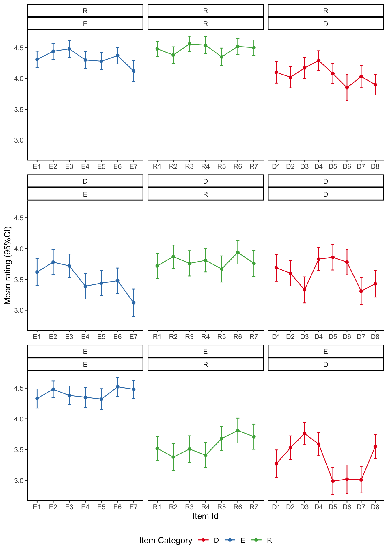
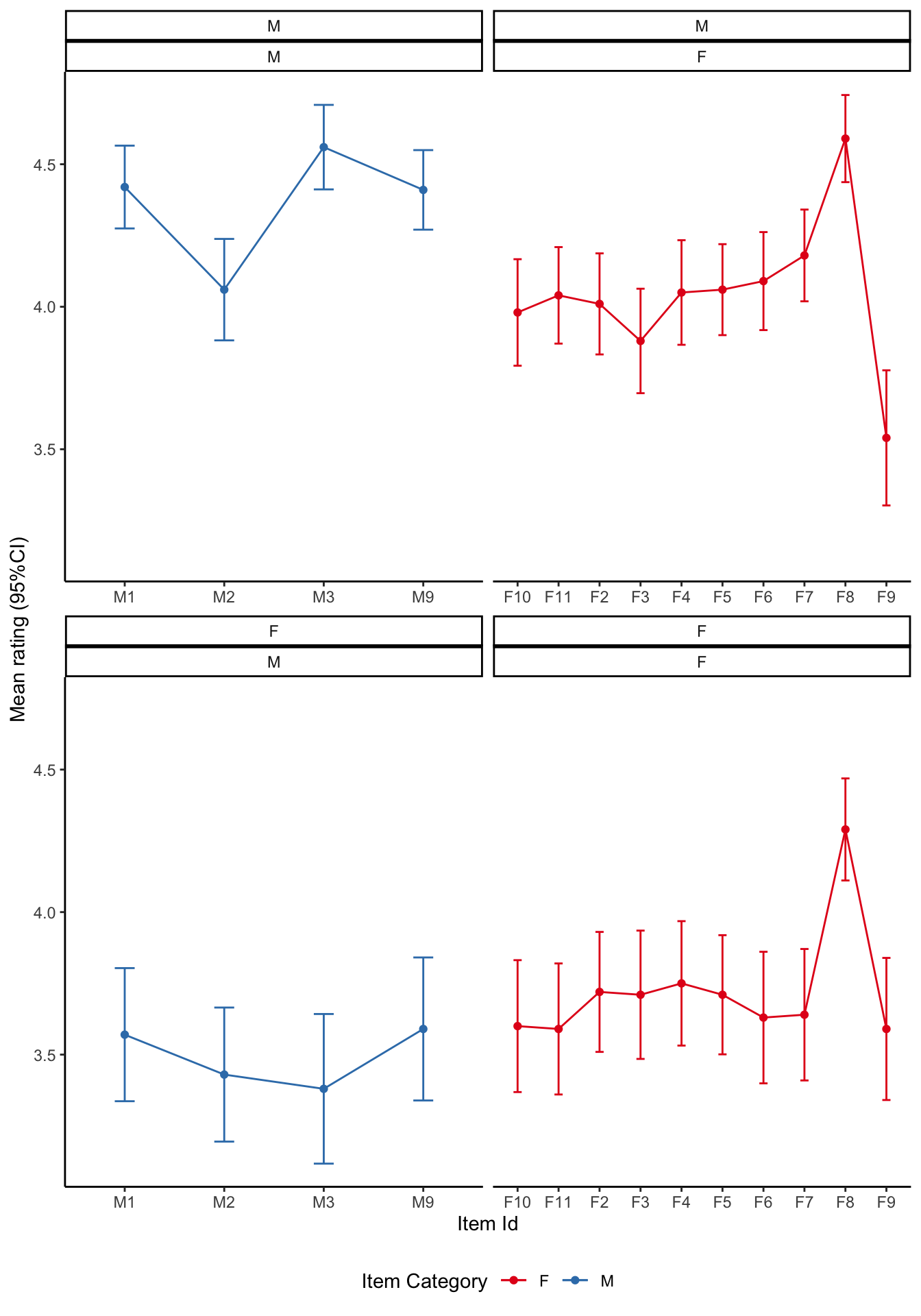
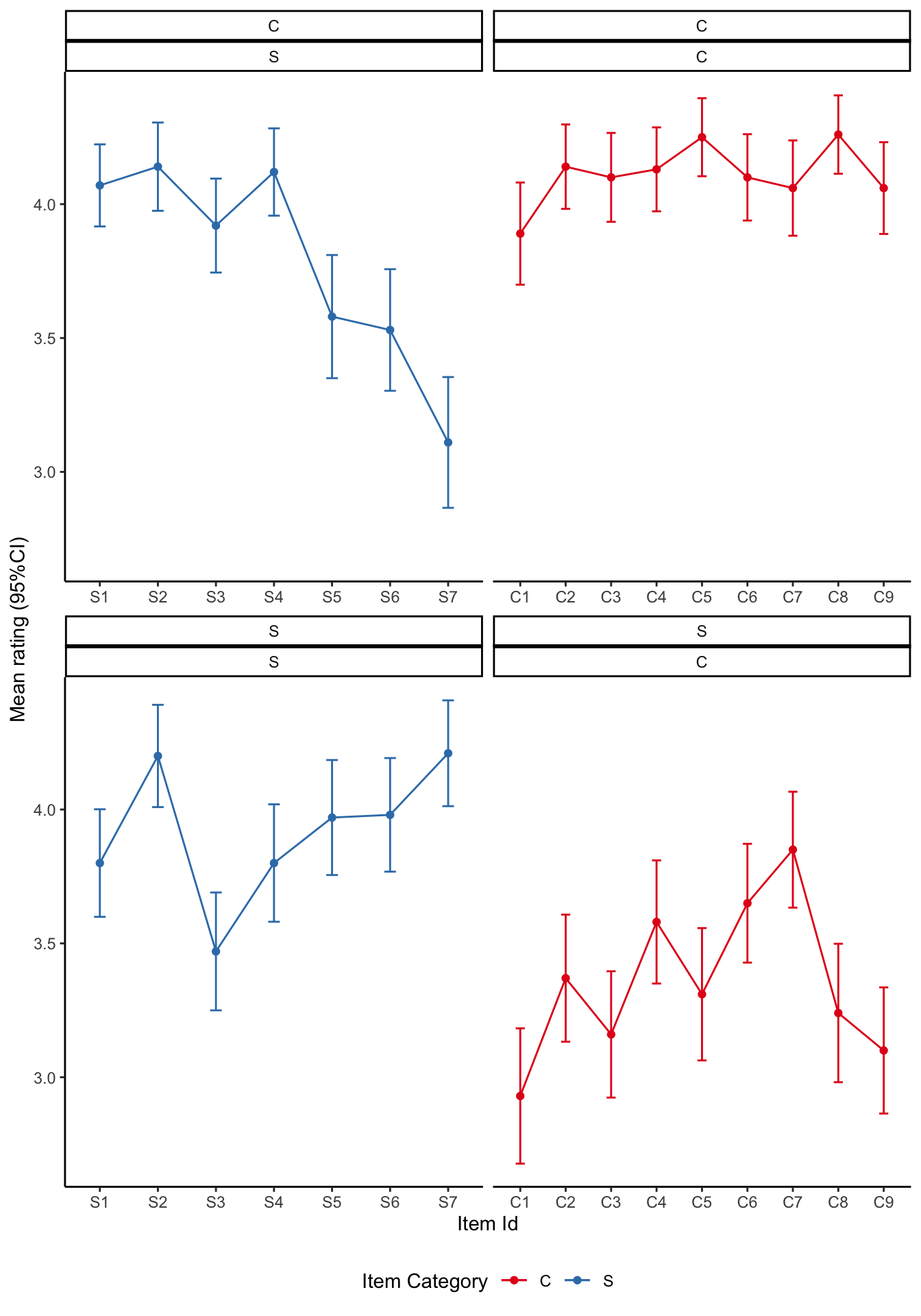
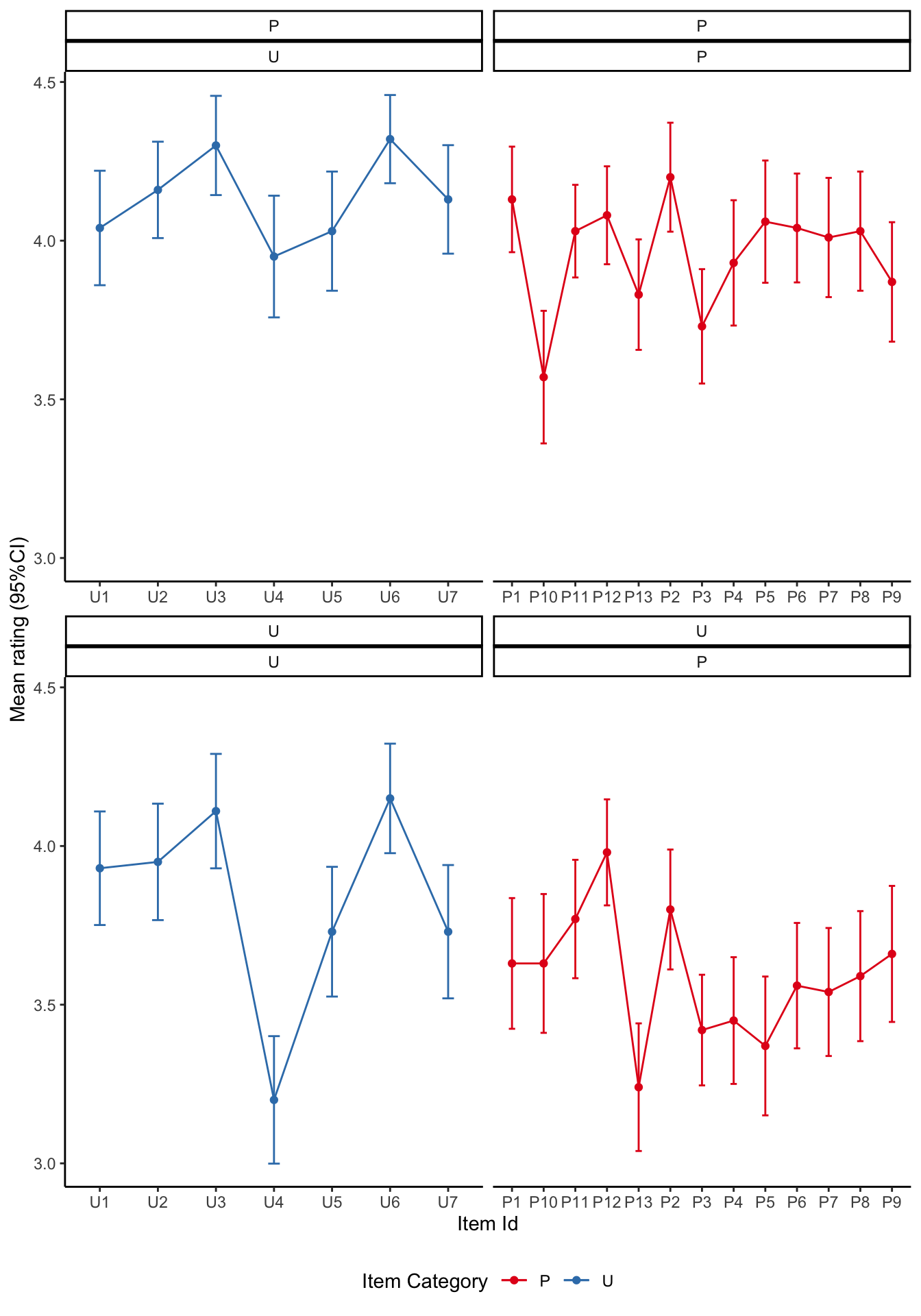
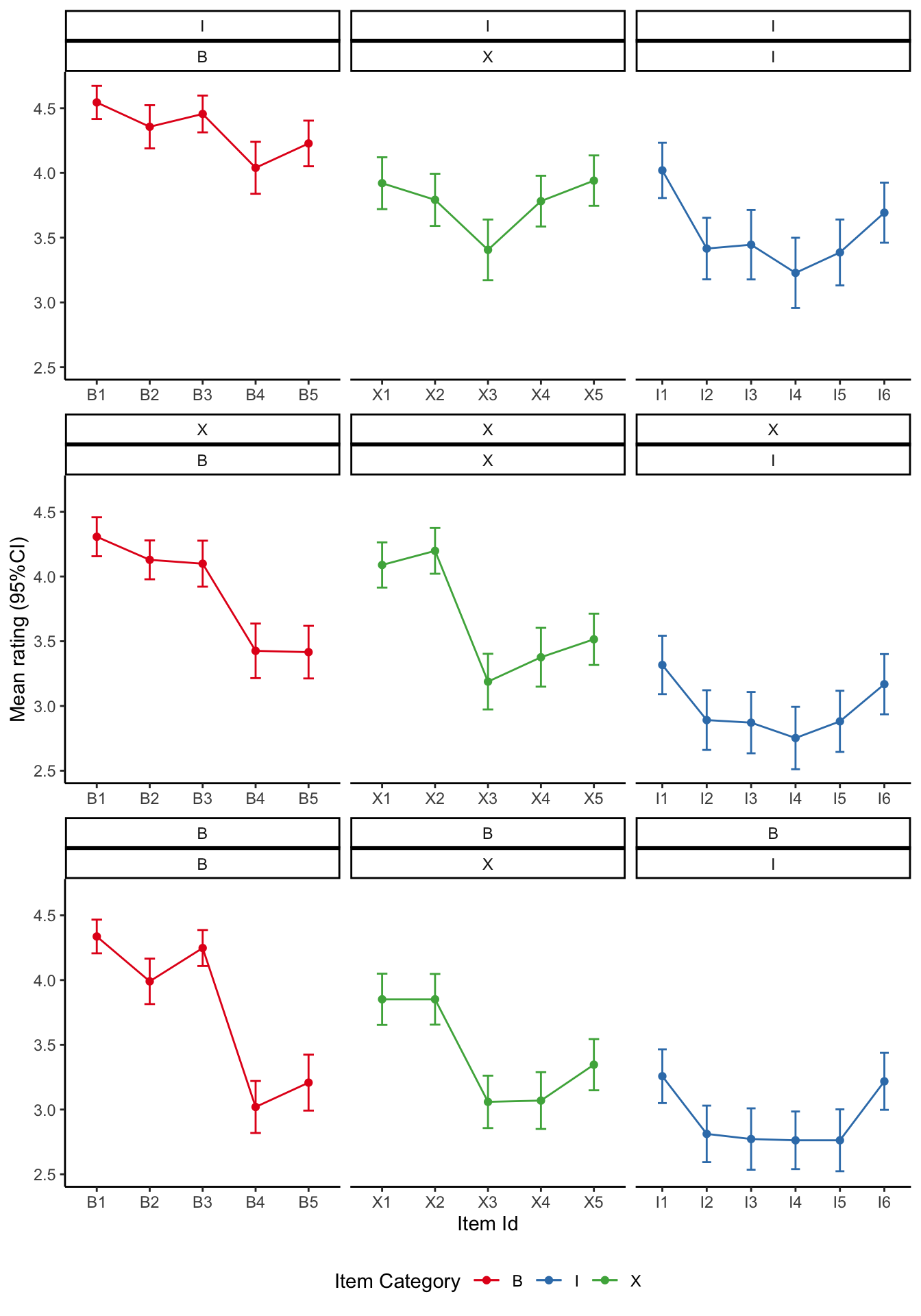
Visualise the mean ratings

source('scr/visualise_means.R')
fig1 <- visualise_means(df1b)

fig2 <- visualise_means(df2b)

fig3 <- visualise_means(df3b)

fig4 <- visualise_means(df4b)

fig5 <- visualise_means(df5b)