This notebook describes the Experiment 2 data : preprocessing, outlier removal, demographics, mean ratings, and distributions. The data in factor study experiment 2 consists of 12 vignettes, with optimised (CFA) 35 items, that utilises between-subject design for vignettes, N=1200 (N=100 for each vignette), with a subset (≈ 50/50%) of participants answering additional questions (GEMIAC N=579, HAAS N=639).
Load and preprocess data
source ('scr/read_EFA_qualtrics.R' ) # custom function source ('scr/convert_items_long.R' ) # custom function source ('scr/participant_reliability.R' ) # custom function #fn <- "data/Episodes_September 9, 2025_14.01.csv" # N=600 GEMIAC #d <- read_EFA_qualtrics(filename = fn,bonusquestion = "GEMIAC") <- "data/Episodes_September 11, 2025_09.14.csv" # N=601-1100 HAAS <- read_EFA_qualtrics (filename = fn,bonusquestion = "HAAS" )<- convert_items_long (d)
[1] "Number of rows in the long data: 43365"
[1] "Number of unique participants in the long data: 1239"
[1] "Number of unique items in the long data: 35"
<- participant_reliability (df,THRESHOLD = 0.001 ,verbose= TRUE )
[1] "------------ Vignette: 1"
[1] "Alpha: 0.97"
[1] "Eliminate the worst participants (r below THRESHOLD)"
[1] "Number of participants to eliminate: 3"
[1] "5687d434369319000c269c03" "59236837989cc20001414f5c"
[3] "613f0ce7ced87b6731521401"
[1] "Alpha: 0.97"
[1] "N after trimming: 1236"
[1] "------------ Vignette: 2"
[1] "Alpha: 0.98"
[1] "Eliminate the worst participants (r below THRESHOLD)"
[1] "No participants to eliminate"
[1] "------------ Vignette: 3"
[1] "Alpha: 0.98"
[1] "Eliminate the worst participants (r below THRESHOLD)"
[1] "Number of participants to eliminate: 3"
[1] "614873a43b76bea1f97ee78f" "6704539fe462b87182866f14"
[3] "676fdad1bc3b61e9e2bd6e30"
[1] "Alpha: 0.98"
[1] "N after trimming: 1233"
[1] "------------ Vignette: 4"
[1] "Alpha: 0.98"
[1] "Eliminate the worst participants (r below THRESHOLD)"
[1] "Number of participants to eliminate: 2"
[1] "651d627dfd76b2f2fb85bf9a" "67d18f41f2533fd38b55a10f"
[1] "Alpha: 0.98"
[1] "N after trimming: 1231"
[1] "------------ Vignette: 5"
[1] "Alpha: 0.97"
[1] "Eliminate the worst participants (r below THRESHOLD)"
[1] "Number of participants to eliminate: 8"
[1] "675cca3a27cd0a6fc7c16a9a" "66a50183d6f19b4257015e67"
[3] "660a6b953836d16312814993" "6606d4f4acdc3a6b8200c0ee"
[5] "5cc9df34a0289a001408c402" "663ccb353b6d9966bcce762a"
[7] "672aa0507fcf257b1477aa72" "5e0fdde8b638537085d51b6c"
[1] "Alpha: 0.98"
[1] "N after trimming: 1223"
[1] "------------ Vignette: 6"
[1] "Alpha: 0.97"
[1] "Eliminate the worst participants (r below THRESHOLD)"
[1] "Number of participants to eliminate: 1"
[1] "66cc6eb364154a51d4d44eb1"
[1] "Alpha: 0.97"
[1] "N after trimming: 1222"
[1] "------------ Vignette: 7"
[1] "Alpha: 0.97"
[1] "Eliminate the worst participants (r below THRESHOLD)"
[1] "Number of participants to eliminate: 3"
[1] "5a8f01d95292b80001235d34" "63469c570cfe46f801523b66"
[3] "6551469abe377d3646c6cd6e"
[1] "Alpha: 0.97"
[1] "N after trimming: 1219"
[1] "------------ Vignette: 8"
[1] "Alpha: 0.98"
[1] "Eliminate the worst participants (r below THRESHOLD)"
[1] "Number of participants to eliminate: 3"
[1] "6779b59fcee735f80b55aa62" "5b68c9eb87af310001584803"
[3] "5e695632d40a492070942196"
[1] "Alpha: 0.98"
[1] "N after trimming: 1216"
[1] "------------ Vignette: 9"
[1] "Alpha: 0.96"
[1] "Eliminate the worst participants (r below THRESHOLD)"
[1] "Number of participants to eliminate: 7"
[1] "6116e4eaa383c256f8253754" "608d247fc141c8230ce3ebdc"
[3] "63cd461c5f597e27b2a054fb" "6673e154af89f4f85eaa7c73"
[5] "62d138e361857aef127c9e8b" "614485923ba5c4783abe671e"
[7] "5a031384fe645f0001e9ea24"
[1] "Alpha: 0.96"
[1] "N after trimming: 1209"
[1] "------------ Vignette: 10"
[1] "Alpha: 0.96"
[1] "Eliminate the worst participants (r below THRESHOLD)"
[1] "Number of participants to eliminate: 1"
[1] "6734acb87201d0735d63632c"
[1] "Alpha: 0.96"
[1] "N after trimming: 1208"
[1] "------------ Vignette: 11"
[1] "Alpha: 0.97"
[1] "Eliminate the worst participants (r below THRESHOLD)"
[1] "Number of participants to eliminate: 7"
[1] "5c4f5967aac8be0001716a65" "63b3377ca1ccdfc7cc567503"
[3] "5dcb2bb4ae3b3b814b5fe27d" "679a0366c8793f4845badfd6"
[5] "5987bfb80e411a0001d83837" "5e90a3adb3e1243bdcfaf973"
[7] "609d1ddf6aa3ba55f1bf4267"
[1] "Alpha: 0.97"
[1] "N after trimming: 1201"
[1] "------------ Vignette: 12"
[1] "Alpha: 0.98"
[1] "Eliminate the worst participants (r below THRESHOLD)"
[1] "Number of participants to eliminate: 1"
[1] "637545d6428d85daeedc3df5"
[1] "Alpha: 0.98"
[1] "N after trimming: 1200"
<- df %>% filter (! ProlificID %in% reliability$ removed_participants)
Summarise participant count across sub-experiments (vignettes)
<- summarise (group_by (df_f,VigNro),n= n ()/ 35 ) # divide by no. of items print (knitr:: kable (S))
1
100
2
100
3
100
4
100
5
100
6
100
7
100
8
100
9
100
10
100
11
100
12
100
Demographics
# get only one row per participant <- df_f %>% select (ProlificID, Age, Gender, OMSI,VigNro) %>% distinct ()#### report print (paste ("Age (M):" ,round (mean (demographics$ Age, na.rm= TRUE ),2 )))print (paste ("Age (SD):" ,round (sd (demographics$ Age, na.rm= TRUE ),2 )))print (table (demographics$ Gender))/ nrow (demographics)
           Female              Male        Non-binary Prefer not to say
              606               583                 5                 6
           Female              Male        Non-binary Prefer not to say
      0.505000000       0.485833333       0.004166667       0.005000000
print (table (demographics$ OMSI))
              Nonmusician  Music-loving Nonmusician          Amateur musician
                      232                       737                       166
 Serious amateur musician Semiprofessional musician     Professional musician
                       50                        11                         4
$ OMSI_cat <- factor (demographics$ OMSI,levels = c ("Nonmusician" ,"Music-loving Nonmusician" ,"Amateur musician" ,"Serious amateur musician" ,"Semiprofessional musician" ,"Professional musician" ),labels = c ("Nonmusician" ,"Nonmusician" ,"Musician" ,"Musician" ,"Musician" ,"Musician" ))table (demographics$ OMSI_cat)/ nrow (demographics)
Nonmusician    Musician
     0.8075      0.1925
# subsets table (demographics$ Gender, demographics$ VigNro)
                     1  2  3  4  5  6  7  8  9 10 11 12
  Female            61 52 52 49 48 43 48 56 48 50 46 53
  Male              38 48 45 50 50 56 52 44 51 49 53 47
  Non-binary         1  0  1  0  2  1  0  0  0  0  0  0
  Prefer not to say  0  0  2  1  0  0  0  0  1  1  1  0
chisq.test (table (demographics$ Gender, demographics$ VigNro))
Warning in chisq.test(table(demographics$Gender, demographics$VigNro)):
Chi-squared approximation may be incorrect
    Pearson's Chi-squared test

data:  table(demographics$Gender, demographics$VigNro)
X-squared = 31.772, df = 33, p-value = 0.5282
<- table (demographics$ OMSI_cat, demographics$ VigNro)print (T)
               1  2  3  4  5  6  7  8  9 10 11 12
  Nonmusician 90 90 85 79 82 80 79 74 72 79 77 82
  Musician    10 10 15 21 18 20 21 26 28 21 23 18
chisq.test (table (demographics$ OMSI_cat, demographics$ VigNro))
    Pearson's Chi-squared test

data:  table(demographics$OMSI_cat, demographics$VigNro)
X-squared = 21.76, df = 11, p-value = 0.0263
summary (aov (Age ~ VigNro, data = demographics))
              Df Sum Sq Mean Sq F value Pr(>F)
VigNro         1      5    4.71   0.026  0.871
Residuals   1198 214866  179.35
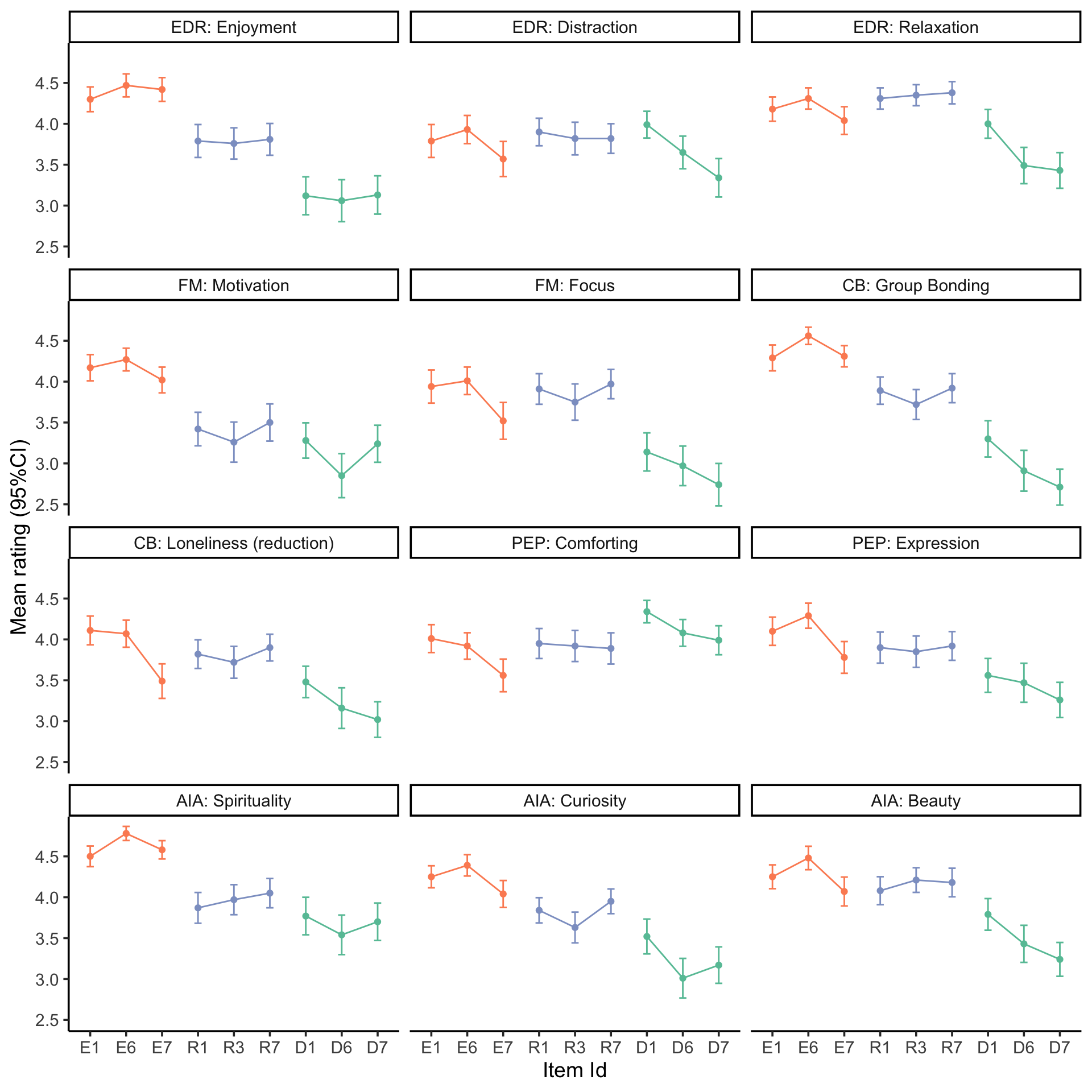
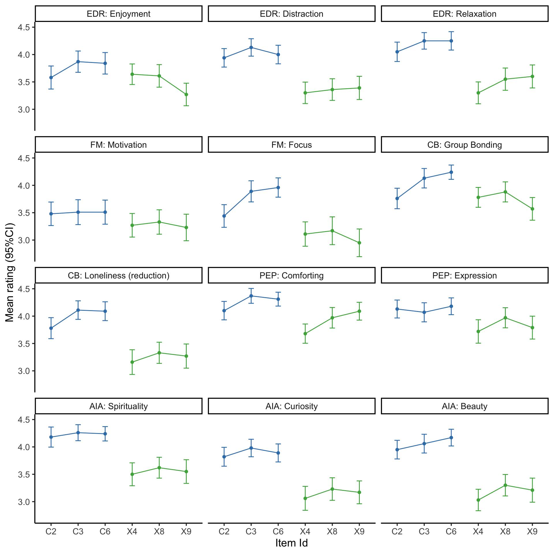
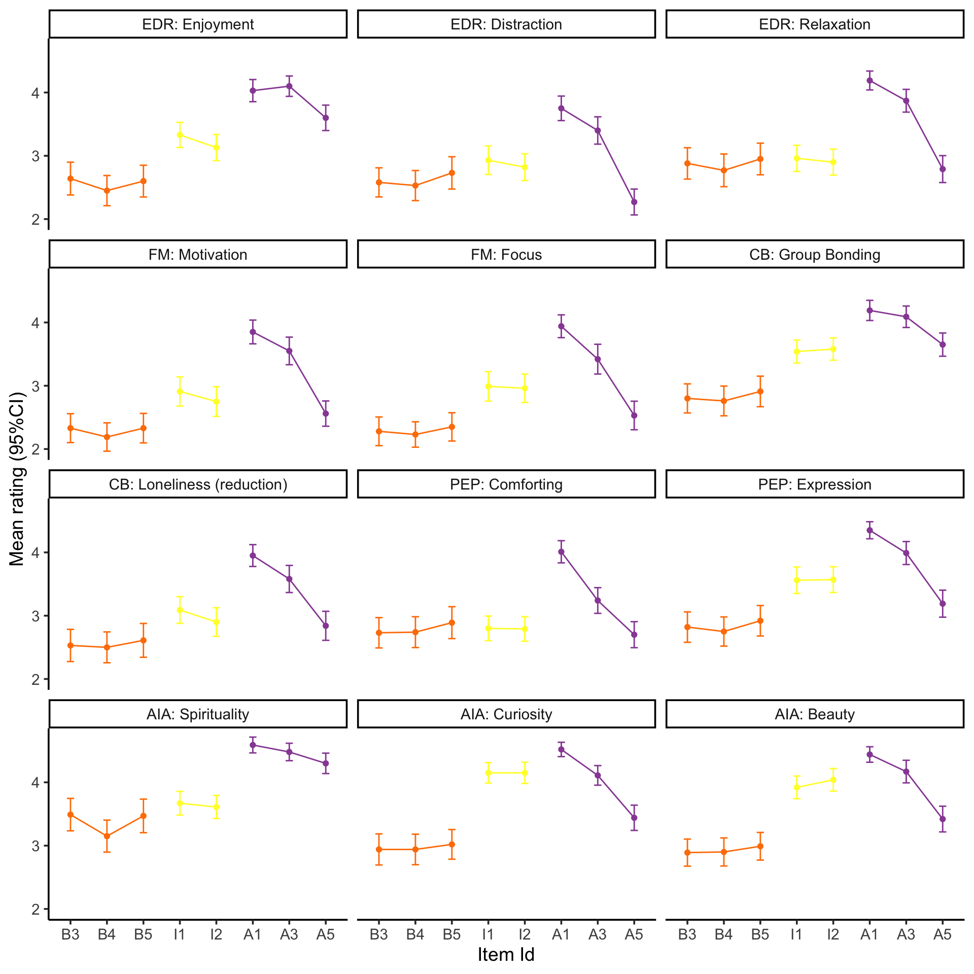
Visualise the mean item ratings
source ('scr/visualise_means.R' )<- NULL 1 ]<- 'EDR: Enjoyment' 2 ]<- 'EDR: Distraction' 3 ]<- 'EDR: Relaxation' 4 ]<- 'FM: Motivation' 5 ]<- 'FM: Focus' 6 ]<- 'CB: Group Bonding' 7 ]<- 'CB: Loneliness (reduction)' 8 ]<- 'PEP: Comforting' 9 ]<- 'PEP: Expression' 10 ]<- 'AIA: Spirituality' 11 ]<- 'AIA: Curiosity' 12 ]<- 'AIA: Beauty' # F1 should be in Motivation, temporarily rename just for figure $ item_label[df_f$ item_label== "F1" ] <- "M9" source ('scr/rename_specific_items.R' ) # We decided to relabel some constructs for clarity <- rename_specific_items (df_f)# Make into a factor $ VigNro <- factor (df_fR$ VigNro,labels= V)$ Construct <- df_fR$ itemCategory
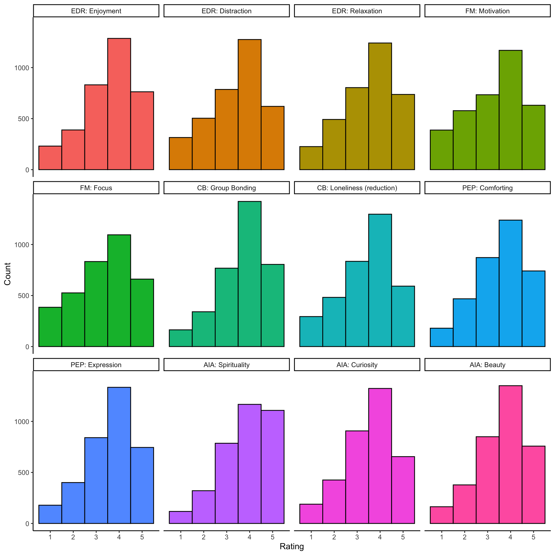
Distributions
Show rating distributions across the vignettes.