library(dmetar,quietly = TRUE)
library(tidyverse,quietly = TRUE)
library(meta)
library(DescTools)
library(ggrepel)
library(forestplot)Analysis
This assumes that the data has been parsed (parse-model-output.R, format-study-results.R) and preprocessed (processing.qmd).
Updated 9/4/2025
Regression studies
Valence
For creating Table 2
Using all models
R_studies <- read.csv("R_studies.csv")
#R_summary <- read.csv("R_summary.csv")

# select regression studies with r2
#tmp <- dplyr::filter(R_summary,dimension=="valence")
tmp <- dplyr::filter(R_studies,dimension=="valence")
#dim(tmp)

#if all studies, remove two with NA values
tmp <- tmp[!is.na(tmp$values),]
#dim(tmp)

# Take all models
m.cor <- metacor(cor = values,     # values
                 n = stimulus_n,
                 studlab = unique_id,
                 data = tmp,
                 common = FALSE,
                 random = TRUE,
                 prediction = TRUE,
#                 backtransf = TRUE,
#                 sm = "ZCOR",
                 method.tau = "PM",# was REML, but we switch to Paule-Mandel because Langan et al., 2019
                 method.random.ci = "HK",
                 title = "MER: Regression: Valence: Summary")

print(m.cor)
Review: MER: Regression: Valence: Summary
Number of studies: k = 102
Number of observations: o = 60017
COR 95%-CI t p-value
Random effects model 0.5832 [0.5410; 0.6226] 21.41 < 0.0001
Prediction interval [0.0552; 0.8563]
Quantifying heterogeneity (with 95%-CIs):
tau^2 = 0.0942 [0.0715; 0.1288]; tau = 0.3070 [0.2674; 0.3589]
I^2 = 97.7% [97.5%; 97.9%]; H = 6.58 [6.28; 6.89]
Test of heterogeneity:
Q d.f. p-value
4371.49 101 0
Details of meta-analysis methods:
- Inverse variance method
- Paule-Mandel estimator for tau^2
- Q-Profile method for confidence interval of tau^2 and tau
- Calculation of I^2 based on Q
- Hartung-Knapp adjustment for random effects model (df = 101)
- Prediction interval based on t-distribution (df = 101)
- Fisher's z transformation of correlationsprint(FisherZInv(m.cor$TE.random))[1] 0.5832415print(FisherZInv(m.cor$upper.random))[1] 0.6225642print(FisherZInv(m.cor$lower.random))[1] 0.5409809Using the best model out of each study
R_summary <- read.csv("R_summary.csv")

# print a summary of features

R_summary |>
  group_by(feature_n_complexity) |>
  summarize(min = min(feature_n),
            max = max(feature_n),
            mean = mean(feature_n),
            mdn = median(feature_n))
# A tibble: 3 × 5
feature_n_complexity min max mean mdn
<chr> <int> <int> <dbl> <dbl>
1 Feature n < 30 3 22 15.7 16.5
2 Feature n > 30 & < 300 45 260 136. 101
3 Feature n > 300 388 14460 3360 654. # select regression studies with r2
tmp <- dplyr::filter(R_summary,dimension=="valence")
#tmp <- dplyr::filter(R_studies,dimension=="valence")
#dim(tmp)
#if all studies, remove two
#tmp <- tmp[!is.na(tmp$values),]
#dim(tmp)
## Disambiguate the studies
tmp$studyREF[tmp$studyREF=="Wang et al 2022"] <- c("Wang et al. 2022a","Wang et al. 2022b")
# Max values
m.cor <- metacor(cor = valuesMax, # values
n = stimulus_n,
studlab = studyREF,#citekey, # unique_id
data = tmp,
common = FALSE,
random = TRUE,
prediction = TRUE,
# backtransf = TRUE,
# sm = "ZCOR",
method.tau = "REML",# could be PM (Paule-Mandel) as well
method.random.ci = "HK",
title = "MER: Regression: Valence: Summary")
print(m.cor)Review: MER: Regression: Valence: Summary
Number of studies: k = 22
Number of observations: o = 14172
COR 95%-CI t p-value
Random effects model 0.6685 [ 0.5599; 0.7546] 9.58 < 0.0001
Prediction interval [-0.0120; 0.9258]
Quantifying heterogeneity (with 95%-CIs):
tau^2 = 0.1484 [0.0847; 0.3121]; tau = 0.3852 [0.2910; 0.5587]
I^2 = 98.4% [98.0%; 98.6%]; H = 7.83 [7.15; 8.58]
Test of heterogeneity:
Q d.f. p-value
1288.63 21 < 0.0001
Details of meta-analysis methods:
- Inverse variance method
- Restricted maximum-likelihood estimator for tau^2
- Q-Profile method for confidence interval of tau^2 and tau
- Calculation of I^2 based on Q
- Hartung-Knapp adjustment for random effects model (df = 21)
- Prediction interval based on t-distribution (df = 21)
- Fisher's z transformation of correlationsprint(FisherZInv(m.cor$TE.random))[1] 0.6685242print(FisherZInv(m.cor$upper.random))[1] 0.7545765print(FisherZInv(m.cor$lower.random))[1] 0.5598682Explore heterogeneity
# Method 1: Give us the Egger's test about beta coefficient from funnel
print(eggers.test(m.cor))
Eggers' test of the intercept
=============================
intercept 95% CI t p
5.05 -0.99 - 11.09 1.637 0.1171758
Eggers' test does not indicate the presence of funnel plot asymmetry. # Method 2: Find the impact to the results when removing those outside the 95CI
O <- find.outliers(m.cor) # 13 remaining out of 24
print(O)Identified outliers (random-effects model)
------------------------------------------
"Battcock et al 2021", "Chen et al 2017", "Coutinho et al 2017", "Griffiths et al 2021", "Hu et al 2017", "Koh et al 2023", "Wang et al. 2022a", "Wang et al. 2022b", "Zhang et al 2019", "Zhang et al 2023"
Results with outliers removed
-----------------------------
Review: MER: Regression: Valence: Summary
Number of studies: k = 12
Number of observations: o = 6150
COR 95%-CI t p-value
Random effects model 0.6855 [0.6346; 0.7306] 20.44 < 0.0001
Prediction interval [0.5143; 0.8042]
Quantifying heterogeneity (with 95%-CIs):
tau^2 = 0.0135 [0.0047; 0.0606]; tau = 0.1164 [0.0682; 0.2461]
I^2 = 82.9% [71.4%; 89.7%]; H = 2.42 [1.87; 3.12]
Test of heterogeneity:
Q d.f. p-value
64.22 11 < 0.0001
Details of meta-analysis methods:
- Inverse variance method
- Restricted maximum-likelihood estimator for tau^2
- Q-Profile method for confidence interval of tau^2 and tau
- Calculation of I^2 based on Q
- Hartung-Knapp adjustment for random effects model (df = 11)
- Prediction interval based on t-distribution (df = 11)
- Fisher's z transformation of correlations# Method 3: Leave-out-out analysis etc for individual influence (not useful here)
#infan <- InfluenceAnalysis(m.cor)
# Method 4: Focus on 10% of most precise studies (Stanley, Jarrel, Doucouliagos 2010)
thres<-quantile(m.cor$seTE,0.1)
ind<-m.cor$seTE<=as.numeric(thres)
m.cor10pct <- update(m.cor, subset = which(ind))
# Method 5: P curve analysis (Simonsohn, Simmons & Nelson, 2015)
pcurve(m.cor)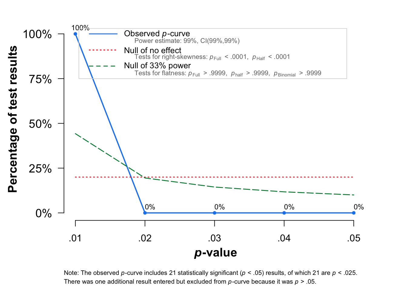
P-curve analysis
 -----------------------
- Total number of provided studies: k = 22
- Total number of p<0.05 studies included into the analysis: k = 21 (95.45%)
- Total number of studies with p<0.025: k = 21 (95.45%)

Results
 -----------------------
                    pBinomial   zFull pFull   zHalf pHalf
Right-skewness test         0 -32.247     0 -31.745     0
Flatness test               1  31.712     1  32.038     1
Note: p-values of 0 or 1 correspond to p<0.001 and p>0.999, respectively.
Power Estimate: 99% (99%-99%)

Evidential value
 -----------------------
- Evidential value present: yes
- Evidential value absent/inadequate: no
Visualise (forest and funnel plots)
fig2a <- meta::forest(m.cor,
       sortvar = TE,
       prediction = FALSE,
             print.tau2 = FALSE,
             leftlabs = c("Author", "N"),studlab = studyREF)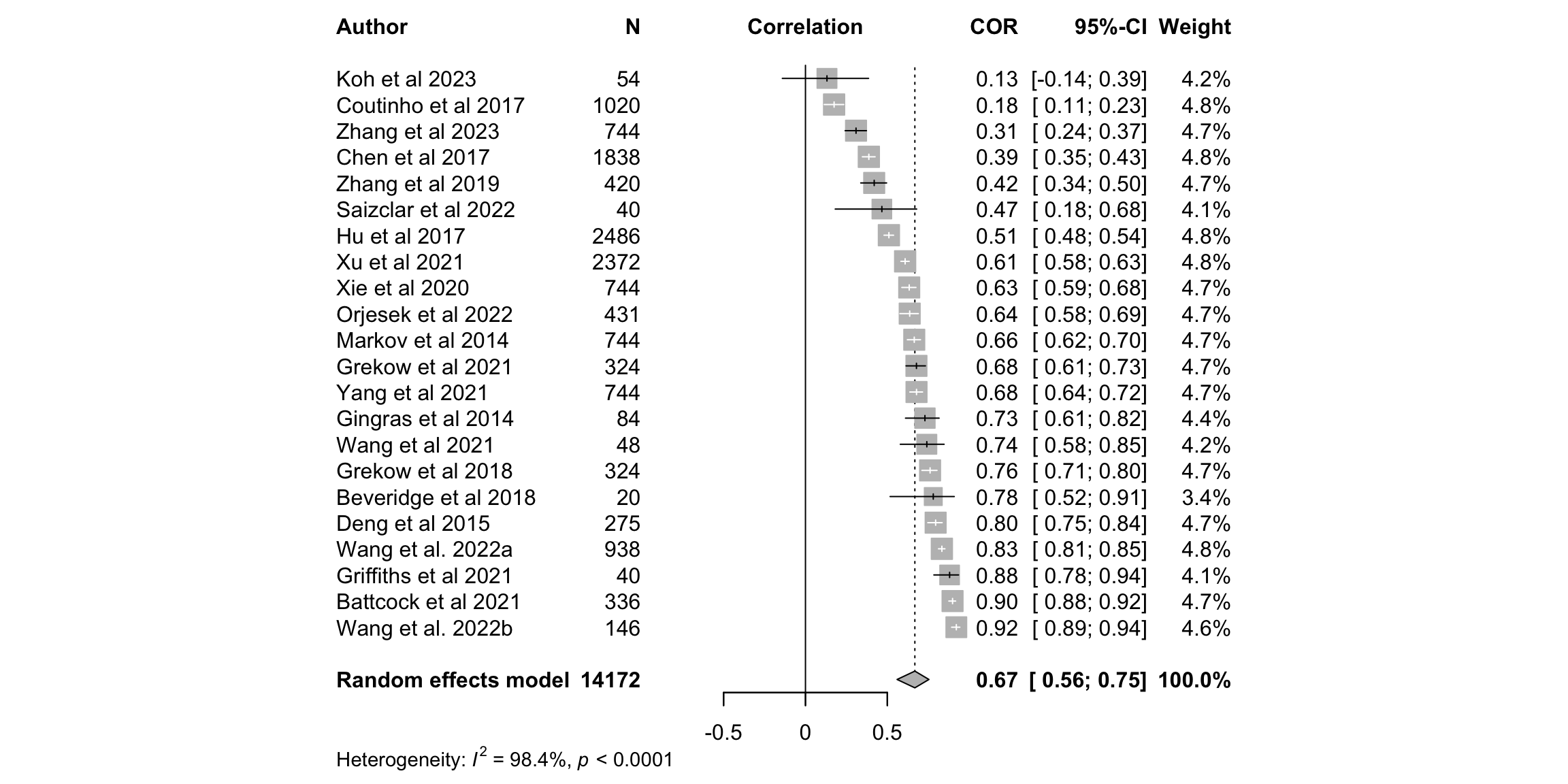
fig2b <- funnel(m.cor, common = FALSE, studlab=TRUE,backtransf=TRUE)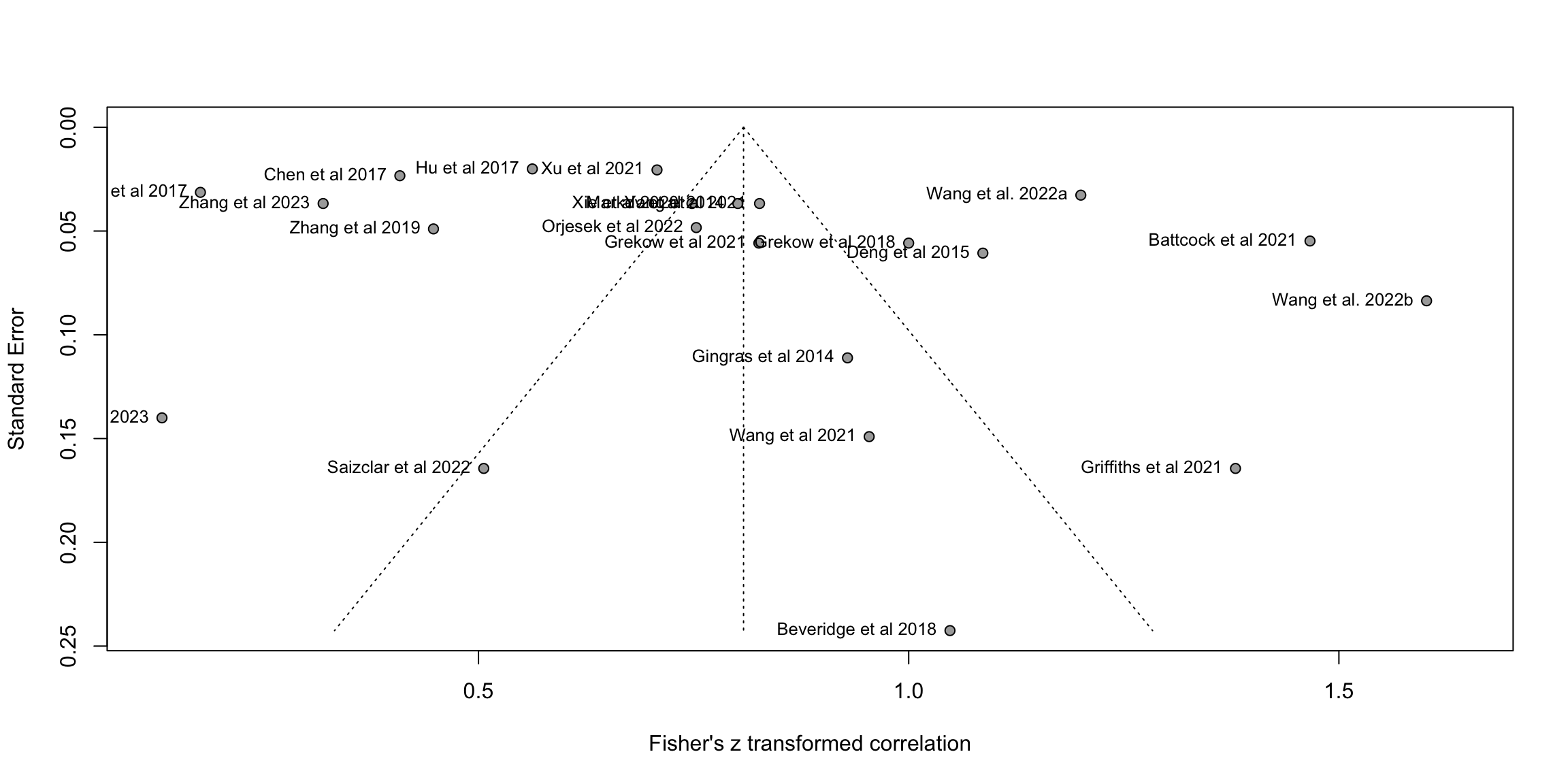
data<-tibble::tibble(mean=m.cor$cor,lower=FisherZInv(m.cor$lower),upper=FisherZInv(m.cor$upper),study=m.cor$studlab,n=m.cor$n,cor=round(m.cor$cor,2))
data<-dplyr::arrange(data,mean)

fp1 <- grid.grabExpr(print(data |>
  forestplot(labeltext = c(study, n, cor),
             xlab = "Correlation",
             xticks = c(0, .25,.5,.75, 1),
             clip = c(0, 1))|>
    fp_add_header(study = "Study",n = "N",cor = expression(italic(r))) |>
    fp_append_row(mean  = m.cor$TE.common,
                lower = m.cor$lower.common,
                upper = m.cor$upper.common,
                study = "Summary",
                n = sum(m.cor$n),
                cor = round(m.cor$TE.common,2),
                is.summary = TRUE) |>
  fp_set_style(box = "grey50",
               line = "grey20",
               summary = "black",
                txt_gp = fpTxtGp(label = list(gpar(cex = 0.80)),
                                ticks = gpar(cex = 0.80),
                                xlab  = gpar(cex = 0.80)))|>
    fp_decorate_graph(grid = structure( m.cor$TE.common,gp = gpar(lty = 2, col = "grey30")))
)
)

source('../etc/custom_funnel_plot.R')
fp2 <- custom_funnel_plot(m.cor)

gridExtra::grid.arrange(fp1, fp2, ncol=2, widths=c(2,1),heights=c(2,1))
Warning: Removed 684 rows containing missing values or values outside the scale range
(`geom_line()`).Warning: Removed 753 rows containing missing values or values outside the scale range
(`geom_line()`).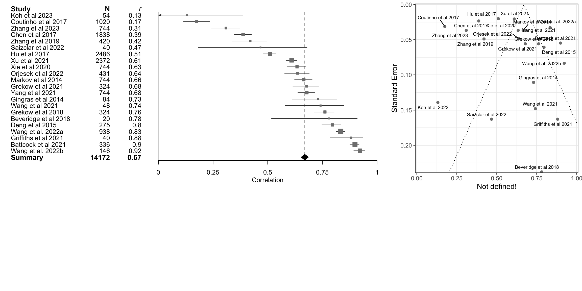
Sub-divisions
Sub-division based on techniques
S <- summarise(group_by(tmp,model_class_id),n=n(),obs=sum(stimulus_n))
print(knitr::kable(S))| model_class_id | n | obs |
|---|---|---|
| Linear Methods | 9 | 2457 |
| Neural Nets | 6 | 3317 |
| Support Vector Machines | 4 | 5068 |
| Tree-based Methods | 3 | 3330 |
m.cor1 <- update(m.cor,
       subgroup = model_class_id)
print(m.cor1)
Review: MER: Regression: Valence: Summary
Number of studies: k = 22
Number of observations: o = 14172
COR 95%-CI t p-value
Random effects model 0.6685 [ 0.5599; 0.7546] 9.58 < 0.0001
Prediction interval [-0.0120; 0.9258]
Quantifying heterogeneity (with 95%-CIs):
tau^2 = 0.1484 [0.0847; 0.3121]; tau = 0.3852 [0.2910; 0.5587]
I^2 = 98.4% [98.0%; 98.6%]; H = 7.83 [7.15; 8.58]
Test of heterogeneity:
Q d.f. p-value
1288.63 21 < 0.0001
Results for subgroups (random effects model):
k COR 95%-CI tau^2
model_class_id = Linear Methods 9 0.7843 [0.6517; 0.8704] 0.1194
model_class_id = Tree-based Methods 3 0.7503 [0.2922; 0.9284] 0.0740
model_class_id = Support Vector Machines 4 0.5386 [0.1714; 0.7744] 0.0702
model_class_id = Neural Nets 6 0.4728 [0.1668; 0.6958] 0.1029
tau Q I^2
model_class_id = Linear Methods 0.3455 214.68 96.3%
model_class_id = Tree-based Methods 0.2721 163.33 98.8%
model_class_id = Support Vector Machines 0.2649 103.27 97.1%
model_class_id = Neural Nets 0.3207 277.64 98.2%
Test for subgroup differences (random effects model):
Q d.f. p-value
Between groups 12.43 3 0.0061
Details of meta-analysis methods:
- Inverse variance method
- Restricted maximum-likelihood estimator for tau^2
- Q-Profile method for confidence interval of tau^2 and tau
- Calculation of I^2 based on Q
- Hartung-Knapp adjustment for random effects model (df = 21)
- Prediction interval based on t-distribution (df = 21)
- Fisher's z transformation of correlationsSub-division based on journals (engineering vs psych)
S <- summarise(group_by(tmp,journal_type),n=n(),obs=sum(stimulus_n))
print(knitr::kable(S))| journal_type | n | obs |
|---|---|---|
| Engineering | 13 | 10002 |
| Psychology | 9 | 4170 |
m.cor2 <- update(m.cor,
       subgroup = journal_type)
print(m.cor2)
Review: MER: Regression: Valence: Summary
Number of studies: k = 22
Number of observations: o = 14172
COR 95%-CI t p-value
Random effects model 0.6685 [ 0.5599; 0.7546] 9.58 < 0.0001
Prediction interval [-0.0120; 0.9258]
Quantifying heterogeneity (with 95%-CIs):
tau^2 = 0.1484 [0.0847; 0.3121]; tau = 0.3852 [0.2910; 0.5587]
I^2 = 98.4% [98.0%; 98.6%]; H = 7.83 [7.15; 8.58]
Test of heterogeneity:
Q d.f. p-value
1288.63 21 < 0.0001
Results for subgroups (random effects model):
k COR 95%-CI tau^2 tau Q
journal_type = Psychology 9 0.6880 [0.4683; 0.8276] 0.1830 0.4278 562.98
journal_type = Engineering 13 0.6564 [0.5052; 0.7685] 0.1378 0.3712 627.09
I^2
journal_type = Psychology 98.6%
journal_type = Engineering 98.1%
Test for subgroup differences (random effects model):
Q d.f. p-value
Between groups 0.10 1 0.7482
Details of meta-analysis methods:
- Inverse variance method
- Restricted maximum-likelihood estimator for tau^2
- Q-Profile method for confidence interval of tau^2 and tau
- Calculation of I^2 based on Q
- Hartung-Knapp adjustment for random effects model (df = 21)
- Prediction interval based on t-distribution (df = 21)
- Fisher's z transformation of correlationsSub-division based on N features
tmp <- dplyr::filter(R_summary,dimension=="valence")
tmp<-tmp[!is.na(tmp$feature_n_complexity),] # remove
S <- summarise(group_by(tmp,feature_n_complexity),n=n(),obs=sum(stimulus_n))
print(knitr::kable(S))| feature_n_complexity | n | obs |
|---|---|---|
| Feature n < 30 | 6 | 3140 |
| Feature n > 30 & < 300 | 8 | 4098 |
| Feature n > 300 | 8 | 6934 |
tmp <- dplyr::filter(R_summary,dimension=="valence")
tmp<-tmp[!is.na(tmp$feature_n_complexity),] # remove missing values
m.cor3 <- update(m.cor,
       subgroup = feature_n_complexity)
print(m.cor3)
Review: MER: Regression: Valence: Summary
Number of studies: k = 22
Number of observations: o = 14172
COR 95%-CI t p-value
Random effects model 0.6685 [ 0.5599; 0.7546] 9.58 < 0.0001
Prediction interval [-0.0120; 0.9258]
Quantifying heterogeneity (with 95%-CIs):
tau^2 = 0.1484 [0.0847; 0.3121]; tau = 0.3852 [0.2910; 0.5587]
I^2 = 98.4% [98.0%; 98.6%]; H = 7.83 [7.15; 8.58]
Test of heterogeneity:
Q d.f. p-value
1288.63 21 < 0.0001
Results for subgroups (random effects model):
k COR 95%-CI
feature_n_complexity = Feature n < 30 6 0.7661 [0.4884; 0.9029]
feature_n_complexity = Feature n > 30 & < 300 8 0.5798 [0.2759; 0.7783]
feature_n_complexity = Feature n > 300 8 0.6657 [0.5314; 0.7673]
tau^2 tau Q I^2
feature_n_complexity = Feature n < 30 0.1976 0.4445 365.94 98.6%
feature_n_complexity = Feature n > 30 & < 300 0.1884 0.4341 271.54 97.4%
feature_n_complexity = Feature n > 300 0.0622 0.2494 353.50 98.0%
Test for subgroup differences (random effects model):
Q d.f. p-value
Between groups 2.03 2 0.3632
Details of meta-analysis methods:
- Inverse variance method
- Restricted maximum-likelihood estimator for tau^2
- Q-Profile method for confidence interval of tau^2 and tau
- Calculation of I^2 based on Q
- Hartung-Knapp adjustment for random effects model (df = 21)
- Prediction interval based on t-distribution (df = 21)
- Fisher's z transformation of correlationsS<-summarise(group_by(tmp,feature_n_complexity),n=n(),obs=sum(stimulus_n))
print(S)# A tibble: 3 × 3
feature_n_complexity n obs
<chr> <int> <int>
1 Feature n < 30 6 3140
2 Feature n > 30 & < 300 8 4098
3 Feature n > 300 8 6934Sub-division based on N features and genres
tmp <- dplyr::filter(R_summary,dimension=="valence")
tmp<-tmp[!is.na(tmp$feature_n_complexity),] # removemissing values

S<-summarise(group_by(tmp,stimulus_genre_mixed),n=n(),obs=sum(stimulus_n))
print(knitr::kable(S))| stimulus_genre_mixed | n | obs |
|---|---|---|
| MultiGenre | 14 | 8787 |
| SingleGenre | 8 | 5385 |
m.cor4 <- update(m.cor,
       subgroup = stimulus_genre_mixed)

print(m.cor4)
Review: MER: Regression: Valence: Summary
Number of studies: k = 22 Number of observations: o = 14172
COR 95%-CI t p-valueRandom effects model 0.6685 [ 0.5599; 0.7546] 9.58 < 0.0001 Prediction interval [-0.0120; 0.9258]
Quantifying heterogeneity (with 95%-CIs): tau^2 = 0.1484 [0.0847; 0.3121]; tau = 0.3852 [0.2910; 0.5587] I^2 = 98.4% [98.0%; 98.6%]; H = 7.83 [7.15; 8.58]
Test of heterogeneity: Q d.f. p-value 1288.63 21 < 0.0001
Results for subgroups (random effects model): k COR 95%-CI tau^2 tau stimulus_genre_mixed = SingleGenre 8 0.6752 [0.4651; 0.8132] 0.1374 0.3707 stimulus_genre_mixed = MultiGenre 14 0.6650 [0.5078; 0.7793] 0.1665 0.4080 Q I^2 stimulus_genre_mixed = SingleGenre 415.17 98.3% stimulus_genre_mixed = MultiGenre 871.51 98.5%
Test for subgroup differences (random effects model): Q d.f. p-value Between groups 0.01 1 0.9158
Details of meta-analysis methods: - Inverse variance method - Restricted maximum-likelihood estimator for tau^2 - Q-Profile method for confidence interval of tau^2 and tau - Calculation of I^2 based on Q - Hartung-Knapp adjustment for random effects model (df = 21) - Prediction interval based on t-distribution (df = 21) - Fisher’s z transformation of correlations
Arousal
Using all models
R_studies <- read.csv("R_studies.csv")
tmp <- dplyr::filter(R_studies,dimension=="arousal")
#if all studies, remove two with NA values
tmp <- tmp[!is.na(tmp$values),]
#dim(tmp)

# Take all models
m.cor <- metacor(cor = values,     # values
                 n = stimulus_n,
                 studlab = unique_id,
                 data = tmp,
                 common = FALSE,
                 random = TRUE,
                 prediction = TRUE,
#                 backtransf = TRUE,
#                 sm = "ZCOR",
                 method.tau = "PM",# was REML, but we switch to Paule-Mandel because Langan et al., 2019
                 method.random.ci = "HK",
                 title = "MER: Regression: Arousal: Summary")

print(m.cor)
Review: MER: Regression: Arousal: Summary
Number of studies: k = 102
Number of observations: o = 60017
COR 95%-CI t p-value
Random effects model 0.7909 [0.7700; 0.8101] 39.90 < 0.0001
Prediction interval [0.4999; 0.9214]
Quantifying heterogeneity (with 95%-CIs):
tau^2 = 0.0692 [0.0520; 0.0955]; tau = 0.2631 [0.2280; 0.3090]
I^2 = 96.2% [95.8%; 96.6%]; H = 5.14 [4.87; 5.43]
Test of heterogeneity:
Q d.f. p-value
2666.55 101 0
Details of meta-analysis methods:
- Inverse variance method
- Paule-Mandel estimator for tau^2
- Q-Profile method for confidence interval of tau^2 and tau
- Calculation of I^2 based on Q
- Hartung-Knapp adjustment for random effects model (df = 101)
- Prediction interval based on t-distribution (df = 101)
- Fisher's z transformation of correlationsprint(FisherZInv(m.cor$TE.random))[1] 0.7908857print(FisherZInv(m.cor$upper.random))[1] 0.8100518print(FisherZInv(m.cor$lower.random))[1] 0.7700316Using the best model out of each study
R_summary <- read.csv("R_summary.csv")

# select regression studies with r2
tmp <- dplyr::filter(R_summary,dimension=="arousal")
#tmp <- dplyr::filter(R_studies,dimension=="valence")
#dim(tmp)

#if all studies, remove two
#tmp <- tmp[!is.na(tmp$values),]
#dim(tmp)

## Disambiguate the studies
tmp$studyREF[tmp$studyREF=="Wang et al 2022"] <- c("Wang et al. 2022a","Wang et al. 2022b")

# Max values
m.cor <- metacor(cor = valuesMax,     # values
                 n = stimulus_n,
                 studlab = studyREF,#citekey, # unique_id
                 data = tmp,
                 common = FALSE,
                 random = TRUE,
                 prediction = TRUE,
#                 backtransf = TRUE,
#                 sm = "ZCOR",
                 method.tau = "REML",# could be PM (Paule-Mandel) as well
                 method.random.ci = "HK",
                 title = "MER: Regression: Arousal: Summary")

print(m.cor)
Review: MER: Regression: Arousal: Summary
Number of studies: k = 22
Number of observations: o = 14172
COR 95%-CI t p-value
Random effects model 0.8087 [0.7404; 0.8604] 13.60 < 0.0001
Prediction interval [0.3127; 0.9582]
Quantifying heterogeneity (with 95%-CIs):
tau^2 = 0.1411 [0.0805; 0.2999]; tau = 0.3756 [0.2838; 0.5476]
I^2 = 97.9% [97.4%; 98.3%]; H = 6.90 [6.26; 7.62]
Test of heterogeneity:
Q d.f. p-value
1001.16 21 < 0.0001
Details of meta-analysis methods:
- Inverse variance method
- Restricted maximum-likelihood estimator for tau^2
- Q-Profile method for confidence interval of tau^2 and tau
- Calculation of I^2 based on Q
- Hartung-Knapp adjustment for random effects model (df = 21)
- Prediction interval based on t-distribution (df = 21)
- Fisher's z transformation of correlationsprint(FisherZInv(m.cor$TE.random))[1] 0.8086765print(FisherZInv(m.cor$upper.random))[1] 0.8604211print(FisherZInv(m.cor$lower.random))[1] 0.7404257Explore heterogeneity
# Method 1: Give us the Egger's test about beta coefficient from funnel
print(eggers.test(m.cor))
Eggers' test of the intercept
=============================
intercept 95% CI t p
0.789 -4.87 - 6.45 0.273 0.7876923
Eggers' test does not indicate the presence of funnel plot asymmetry. # Method 2: Find the impact to the results when removing those outside the 95CI
O <- find.outliers(m.cor) # 13 remaining out of 24
print(O)Identified outliers (random-effects model)
------------------------------------------
"Battcock et al 2021", "Coutinho et al 2017", "Gingras et al 2014", "Grekow et al 2018", "Koh et al 2023", "Orjesek et al 2022", "Wang et al. 2022b", "Zhang et al 2019", "Zhang et al 2023"
Results with outliers removed
-----------------------------
Review: MER: Regression: Arousal: Summary
Number of studies: k = 13
Number of observations: o = 10613
COR 95%-CI t p-value
Random effects model 0.8262 [0.8061; 0.8445] 42.44 < 0.0001
Prediction interval [0.7721; 0.8684]
Quantifying heterogeneity (with 95%-CIs):
tau^2 = 0.0042 [0.0016; 0.0501]; tau = 0.0649 [0.0401; 0.2239]
I^2 = 76.8% [60.6%; 86.4%]; H = 2.08 [1.59; 2.71]
Test of heterogeneity:
Q d.f. p-value
51.82 12 < 0.0001
Details of meta-analysis methods:
- Inverse variance method
- Restricted maximum-likelihood estimator for tau^2
- Q-Profile method for confidence interval of tau^2 and tau
- Calculation of I^2 based on Q
- Hartung-Knapp adjustment for random effects model (df = 12)
- Prediction interval based on t-distribution (df = 12)
- Fisher's z transformation of correlations# Method 3: Leave-out-out analysis etc for individual influence (not useful here)
#infan <- InfluenceAnalysis(m.cor)
# Method 4: Focus on 10% of most precise studies (Stanley, Jarrel, Doucouliagos 2010)
thres<-quantile(m.cor$seTE,0.1)
ind<-m.cor$seTE<=as.numeric(thres)
m.cor10pct <- update(m.cor, subset = which(ind))
# Method 5: P curve analysis (Simonsohn, Simmons & Nelson, 2015)
pcurve(m.cor)
P-curve analysis
 -----------------------
- Total number of provided studies: k = 22
- Total number of p<0.05 studies included into the analysis: k = 22 (100%)
- Total number of studies with p<0.025: k = 22 (100%)

Results
 -----------------------
                    pBinomial   zFull pFull   zHalf pHalf
Right-skewness test         0 -33.770     0 -33.237     0
Flatness test               1  34.184     1  34.443     1
Note: p-values of 0 or 1 correspond to p<0.001 and p>0.999, respectively.
Power Estimate: 99% (99%-99%)

Evidential value
 -----------------------
- Evidential value present: yes
- Evidential value absent/inadequate: no
Visualise (forest and funnel plots)
fig2a <- forest(m.cor,
       sortvar = TE,
       prediction = FALSE,
             print.tau2 = FALSE,
             leftlabs = c("Author", "N"),studlab = studyREF)
fig2b<-funnel(m.cor, common = FALSE, studlab=TRUE,backtransf=TRUE)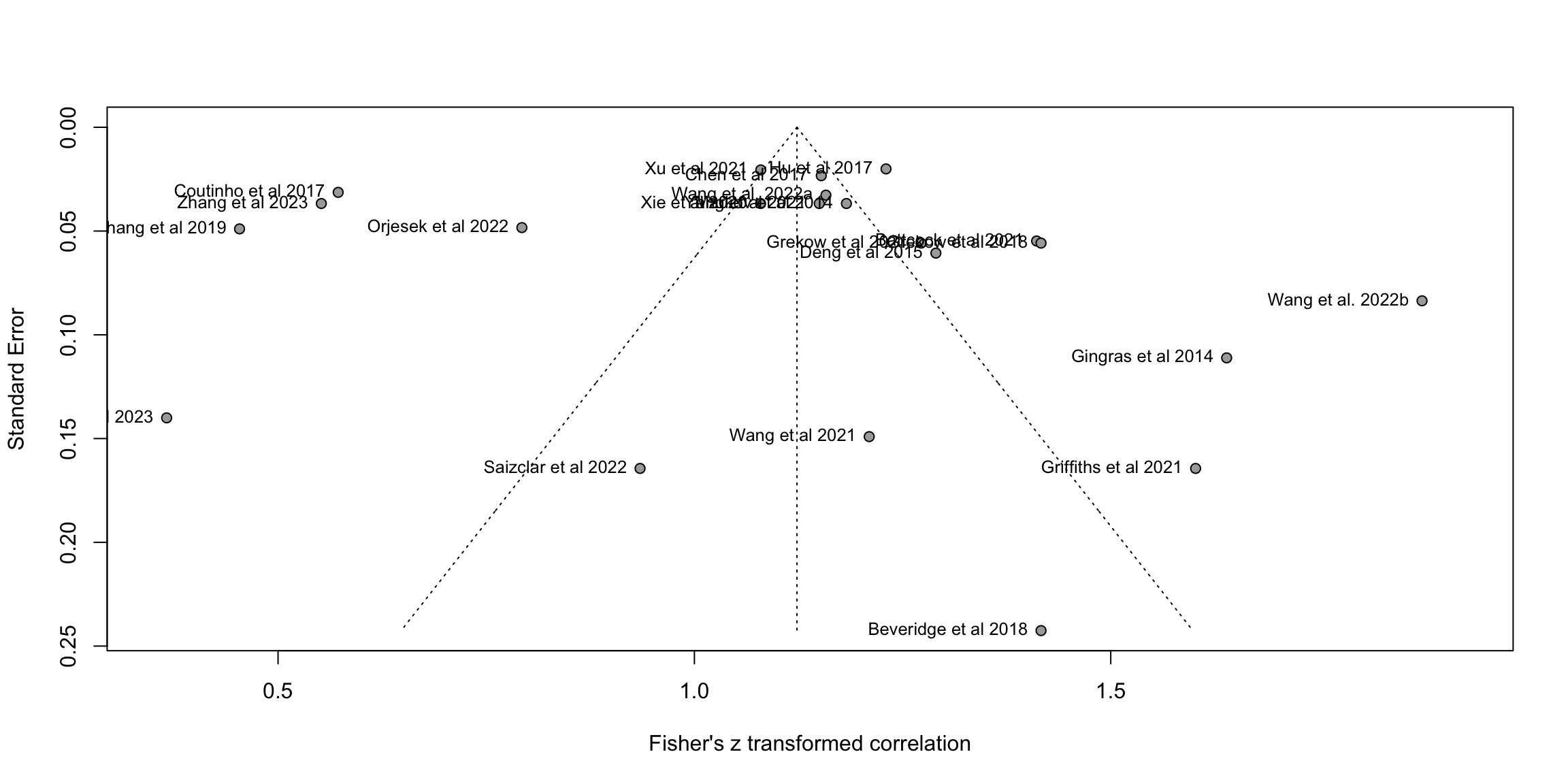
data<-tibble::tibble(mean=m.cor$cor,lower=FisherZInv(m.cor$lower),upper=FisherZInv(m.cor$upper),study=m.cor$studlab,n=m.cor$n,cor=round(m.cor$cor,2))
data<-dplyr::arrange(data,mean)

fp1 <- grid.grabExpr(print(data |>
  forestplot(labeltext = c(study, n, cor),
             xlab = "Correlation",
             xticks = c(0, .25,.5,.75, 1),
             clip = c(0, 1))|>
    fp_add_header(study = "Study",n = "N",cor = expression(italic(r))) |>
    fp_append_row(mean  = m.cor$TE.common,
                lower = m.cor$lower.common,
                upper = m.cor$upper.common,
                study = "Summary",
                n = sum(m.cor$n),
                cor = round(m.cor$TE.common,2),
                is.summary = TRUE) |>
  fp_set_style(box = "grey50",
               line = "grey20",
               summary = "black",
                txt_gp = fpTxtGp(label = list(gpar(cex = 0.80)),
                                ticks = gpar(cex = 0.80),
                                xlab  = gpar(cex = 0.80)))|>
    fp_decorate_graph(grid = structure( m.cor$TE.common,gp = gpar(lty = 2, col = "grey30")))
)
)

source('../etc/custom_funnel_plot.R')
fp2 <- custom_funnel_plot(m.cor)

gridExtra::grid.arrange(fp1, fp2, ncol=2, widths=c(2,1),heights=c(2,1))
Warning: Removed 754 rows containing missing values or values outside the scale range
(`geom_line()`).Warning: Removed 954 rows containing missing values or values outside the scale range
(`geom_line()`).Warning: Removed 1 row containing missing values or values outside the scale range
(`geom_hline()`).
Sub-divisions
Sub-division based on techniques
S <- summarise(group_by(tmp,model_class_id),n=n(),obs=sum(stimulus_n))
print(knitr::kable(S))| model_class_id | n | obs |
|---|---|---|
| Linear Methods | 8 | 1713 |
| Neural Nets | 6 | 3317 |
| Support Vector Machines | 5 | 5812 |
| Tree-based Methods | 3 | 3330 |
m.cor1 <- update(m.cor,
                 subgroup = model_class_id
)
print(m.cor1)
Review: MER: Regression: Arousal: Summary
Number of studies: k = 22
Number of observations: o = 14172
COR 95%-CI t p-value
Random effects model 0.8087 [0.7404; 0.8604] 13.60 < 0.0001
Prediction interval [0.3127; 0.9582]
Quantifying heterogeneity (with 95%-CIs):
tau^2 = 0.1411 [0.0805; 0.2999]; tau = 0.3756 [0.2838; 0.5476]
I^2 = 97.9% [97.4%; 98.3%]; H = 6.90 [6.26; 7.62]
Test of heterogeneity:
Q d.f. p-value
1001.16 21 < 0.0001
Results for subgroups (random effects model):
k COR 95%-CI tau^2
model_class_id = Linear Methods 8 0.8818 [0.8090; 0.9279] 0.0840
model_class_id = Tree-based Methods 3 0.8085 [0.7334; 0.8641] 0.0025
model_class_id = Support Vector Machines 5 0.7959 [0.5590; 0.9127] 0.1325
model_class_id = Neural Nets 6 0.6597 [0.3954; 0.8231] 0.1209
tau Q I^2
model_class_id = Linear Methods 0.2898 104.84 93.3%
model_class_id = Tree-based Methods 0.0505 5.77 65.4%
model_class_id = Support Vector Machines 0.3640 241.54 98.3%
model_class_id = Neural Nets 0.3477 270.03 98.1%
Test for subgroup differences (random effects model):
Q d.f. p-value
Between groups 10.83 3 0.0127
Details of meta-analysis methods:
- Inverse variance method
- Restricted maximum-likelihood estimator for tau^2
- Q-Profile method for confidence interval of tau^2 and tau
- Calculation of I^2 based on Q
- Hartung-Knapp adjustment for random effects model (df = 21)
- Prediction interval based on t-distribution (df = 21)
- Fisher's z transformation of correlationsSub-division based on journals (engineering vs psych)
S <- summarise(group_by(tmp,journal_type),n=n(),obs=sum(stimulus_n))
print(knitr::kable(S))| journal_type | n | obs |
|---|---|---|
| Engineering | 13 | 10002 |
| Psychology | 9 | 4170 |
m.cor2 <- update(
  m.cor,
  subgroup = journal_type
)
print(m.cor2)
Review: MER: Regression: Arousal: Summary
Number of studies: k = 22
Number of observations: o = 14172
COR 95%-CI t p-value
Random effects model 0.8087 [0.7404; 0.8604] 13.60 < 0.0001
Prediction interval [0.3127; 0.9582]
Quantifying heterogeneity (with 95%-CIs):
tau^2 = 0.1411 [0.0805; 0.2999]; tau = 0.3756 [0.2838; 0.5476]
I^2 = 97.9% [97.4%; 98.3%]; H = 6.90 [6.26; 7.62]
Test of heterogeneity:
Q d.f. p-value
1001.16 21 < 0.0001
Results for subgroups (random effects model):
k COR 95%-CI tau^2 tau Q
journal_type = Psychology 9 0.8389 [0.7417; 0.9016] 0.1079 0.3286 345.30
journal_type = Engineering 13 0.7858 [0.6693; 0.8647] 0.1655 0.4068 650.86
I^2
journal_type = Psychology 97.7%
journal_type = Engineering 98.2%
Test for subgroup differences (random effects model):
Q d.f. p-value
Between groups 0.94 1 0.3332
Details of meta-analysis methods:
- Inverse variance method
- Restricted maximum-likelihood estimator for tau^2
- Q-Profile method for confidence interval of tau^2 and tau
- Calculation of I^2 based on Q
- Hartung-Knapp adjustment for random effects model (df = 21)
- Prediction interval based on t-distribution (df = 21)
- Fisher's z transformation of correlationsSub-division based on N features
tmp <- dplyr::filter(R_summary,dimension=="arousal")
tmp<-tmp[!is.na(tmp$feature_n_complexity),] # remove
S <- summarise(group_by(tmp,feature_n_complexity),n=n(),obs=sum(stimulus_n))
print(knitr::kable(S))| feature_n_complexity | n | obs |
|---|---|---|
| Feature n < 30 | 6 | 3140 |
| Feature n > 30 & < 300 | 8 | 4098 |
| Feature n > 300 | 8 | 6934 |
tmp <- dplyr::filter(R_summary,dimension=="arousal")
tmp<-tmp[!is.na(tmp$feature_n_complexity),] # remove missing values
m.cor3 <- update(
  m.cor,
  subgroup = feature_n_complexity
)
print(m.cor3)
Review: MER: Regression: Arousal: Summary
Number of studies: k = 22
Number of observations: o = 14172
COR 95%-CI t p-value
Random effects model 0.8087 [0.7404; 0.8604] 13.60 < 0.0001
Prediction interval [0.3127; 0.9582]
Quantifying heterogeneity (with 95%-CIs):
tau^2 = 0.1411 [0.0805; 0.2999]; tau = 0.3756 [0.2838; 0.5476]
I^2 = 97.9% [97.4%; 98.3%]; H = 6.90 [6.26; 7.62]
Test of heterogeneity:
Q d.f. p-value
1001.16 21 < 0.0001
Results for subgroups (random effects model):
k COR 95%-CI
feature_n_complexity = Feature n < 30 6 0.8845 [0.7818; 0.9404]
feature_n_complexity = Feature n > 30 & < 300 8 0.7347 [0.5012; 0.8684]
feature_n_complexity = Feature n > 300 8 0.8039 [0.7162; 0.8667]
tau^2 tau Q I^2
feature_n_complexity = Feature n < 30 0.0948 0.3078 77.29 93.5%
feature_n_complexity = Feature n > 30 & < 300 0.1971 0.4440 392.70 98.2%
feature_n_complexity = Feature n > 300 0.0612 0.2474 271.79 97.4%
Test for subgroup differences (random effects model):
Q d.f. p-value
Between groups 5.20 2 0.0741
Details of meta-analysis methods:
- Inverse variance method
- Restricted maximum-likelihood estimator for tau^2
- Q-Profile method for confidence interval of tau^2 and tau
- Calculation of I^2 based on Q
- Hartung-Knapp adjustment for random effects model (df = 21)
- Prediction interval based on t-distribution (df = 21)
- Fisher's z transformation of correlationsS<-summarise(group_by(tmp,feature_n_complexity),n=n(),obs=sum(stimulus_n))
print(S)# A tibble: 3 × 3
feature_n_complexity n obs
<chr> <int> <int>
1 Feature n < 30 6 3140
2 Feature n > 30 & < 300 8 4098
3 Feature n > 300 8 6934Sub-division based on N features and genres
tmp <- dplyr::filter(R_summary,dimension=="arousal")
tmp<-tmp[!is.na(tmp$feature_n_complexity),] # remove missing values

S<-summarise(group_by(tmp,stimulus_genre_mixed),n=n(),obs=sum(stimulus_n))
print(knitr::kable(S))| stimulus_genre_mixed | n | obs |
|---|---|---|
| MultiGenre | 14 | 8787 |
| SingleGenre | 8 | 5385 |
m.cor4 <- update(
  m.cor,
  subgroup = stimulus_genre_mixed
)

print(m.cor4)
Review: MER: Regression: Arousal: Summary
Number of studies: k = 22 Number of observations: o = 14172
COR 95%-CI t p-valueRandom effects model 0.8087 [0.7404; 0.8604] 13.60 < 0.0001 Prediction interval [0.3127; 0.9582]
Quantifying heterogeneity (with 95%-CIs): tau^2 = 0.1411 [0.0805; 0.2999]; tau = 0.3756 [0.2838; 0.5476] I^2 = 97.9% [97.4%; 98.3%]; H = 6.90 [6.26; 7.62]
Test of heterogeneity: Q d.f. p-value 1001.16 21 < 0.0001
Results for subgroups (random effects model): k COR 95%-CI tau^2 tau stimulus_genre_mixed = SingleGenre 8 0.8218 [0.6935; 0.8996] 0.1278 0.3574 stimulus_genre_mixed = MultiGenre 14 0.8010 [0.6987; 0.8712] 0.1587 0.3984 Q I^2 stimulus_genre_mixed = SingleGenre 248.32 97.2% stimulus_genre_mixed = MultiGenre 748.31 98.3%
Test for subgroup differences (random effects model): Q d.f. p-value Between groups 0.13 1 0.7205
Details of meta-analysis methods: - Inverse variance method - Restricted maximum-likelihood estimator for tau^2 - Q-Profile method for confidence interval of tau^2 and tau - Calculation of I^2 based on Q - Hartung-Knapp adjustment for random effects model (df = 21) - Prediction interval based on t-distribution (df = 21) - Fisher’s z transformation of correlations
Classification studies: overall success
C_studies <- read.csv("C_studies.csv")
C_studies <- C_studies[!is.na(C_studies$values),]

# yang2021an needs to be encoded for classification (currently just regression)
C_summary <- read.csv("C_summary.csv")
C_classes <- read.csv("C_study_class_n.csv")

C_summary <- merge(C_summary, C_classes)

# print a summary of features

C_summary |>
  group_by(feature_n_complexity) |>
  summarize(min = min(feature_n),
            max = max(feature_n),
            mean = mean(feature_n),
            mdn = median(feature_n))
# A tibble: 3 × 5
feature_n_complexity min max mean mdn
<chr> <int> <int> <dbl> <dbl>
1 Feature n < 30 6 11 8.75 9
2 Feature n > 30 & < 300 98 231 139. 122
3 Feature n > 300 397 8904 3668. 1702m.cor.c.all <- metacor(cor = values, # values
n = stimulus_n,
studlab = studyREF, # unique_id
data = C_studies,
common = FALSE,
random = TRUE,
prediction = TRUE,
backtransf = TRUE,
sm = "ZCOR",
method.tau = "REML",# could be PM (Paule-Mandel) as well
method.random.ci = "HK",
title = "MER: Classification: Summary")
m.cor.c.allReview: MER: Classification: Summary
Number of studies: k = 86
Number of observations: o = 80544
COR 95%-CI t p-value
Random effects model 0.8245 [0.7904; 0.8535] 23.68 < 0.0001
Prediction interval [0.2525; 0.9695]
Quantifying heterogeneity (with 95%-CIs):
tau^2 = 0.2082 [0.1555; 0.2863]; tau = 0.4563 [0.3943; 0.5351]
I^2 = 99.7%; H = 17.62
Test of heterogeneity:
Q d.f. p-value
26400.08 85 0
Details of meta-analysis methods:
- Inverse variance method
- Restricted maximum-likelihood estimator for tau^2
- Q-Profile method for confidence interval of tau^2 and tau
- Calculation of I^2 based on Q
- Hartung-Knapp adjustment for random effects model (df = 85)
- Prediction interval based on t-distribution (df = 85)
- Fisher's z transformation of correlations#m.cor_backtransformed <- m.cor
#m.cor_backtransformed$TE <- FisherZInv(m.cor_backtransformed$TE)
#print(funnel(m.cor.c.all, common = FALSE, studlab=TRUE,backtransf=TRUE))Define splits for genre & stimulus n combinations
# get stimulus and genre metadata for classification studies:
C_studies |>
  group_by(citekey) |>
  summarize(feature_n = unique(feature_n),
            feature_n_complexity = unique(feature_n_complexity),
            stimulus_genre_mixed = unique(stimulus_genre_mixed)) -> C_splits

# create feature_n_complexity_genre column:
C_splits$feature_n_complexity_genre <- ""

# define splits
C_splits[C_splits$feature_n_complexity %in% "Feature n > 30 & < 300" &
        C_splits$stimulus_genre_mixed == "MultiGenre",]$feature_n_complexity_genre <- "Medium multi-genre study"
C_splits[C_splits$stimulus_genre_mixed %in% "SingleGenre" &
                             C_splits$feature_n_complexity %in% "Feature n < 30" ,]$feature_n_complexity_genre <- "Small single-genre study"
C_splits[C_splits$feature_n_complexity == "Feature n > 300",]$feature_n_complexity_genre <- "Huge single or multigenre study"
C_splits[C_splits$citekey == "alvarez2023ri",]$feature_n_complexity_genre <- "Small, multi-genre study"
C_splits[C_splits$citekey == "zhang2016br",]$feature_n_complexity_genre <- "Medium, single-genre study"
# add splits to summary:
C_summary <- left_join(C_summary, C_splits)
Joining with `by = join_by(citekey, feature_n, feature_n_complexity,
stimulus_genre_mixed)`Define splits for binary vs. multiclass
C_summary$classes <- 0
C_summary[C_summary$n_classes < 3,]$classes <- "Binary"
C_summary[C_summary$n_classes >= 3,]$classes <- "Multiclass"
Classification models: best models
m.cor.c <- metacor(cor = valuesMax,     # values
                 n = stimulus_n,
                 studlab = studyREF, # unique_id
                 data = C_summary,
                 common = FALSE,
                 random = TRUE,
                 prediction = TRUE,
                 backtransf = TRUE,
                 sm = "ZCOR",
                 method.tau = "REML",# could be PM (Paule-Mandel) as well
                 method.random.ci = "HK",
                 title = "MER: Classification: Summary")

print(m.cor.c)
Review: MER: Classification: Summary
Number of studies: k = 12
Number of observations: o = 15696
COR 95%-CI t p-value
Random effects model 0.8684 [0.7475; 0.9336] 8.13 < 0.0001
Prediction interval [0.0341; 0.9894]
Quantifying heterogeneity (with 95%-CIs):
tau^2 = 0.3180 [0.1582; 0.9169]; tau = 0.5639 [0.3977; 0.9576]
I^2 = 99.8%; H = 21.39
Test of heterogeneity:
Q d.f. p-value
5031.22 11 0
Details of meta-analysis methods:
- Inverse variance method
- Restricted maximum-likelihood estimator for tau^2
- Q-Profile method for confidence interval of tau^2 and tau
- Calculation of I^2 based on Q
- Hartung-Knapp adjustment for random effects model (df = 11)
- Prediction interval based on t-distribution (df = 11)
- Fisher's z transformation of correlationsCustom funnel for classification studies
fig3a <- forest(m.cor.c,
                sortvar = TE,
                prediction = FALSE,
                print.tau2 = FALSE,
                leftlabs = c("Author", "N"),studlab = studyREF)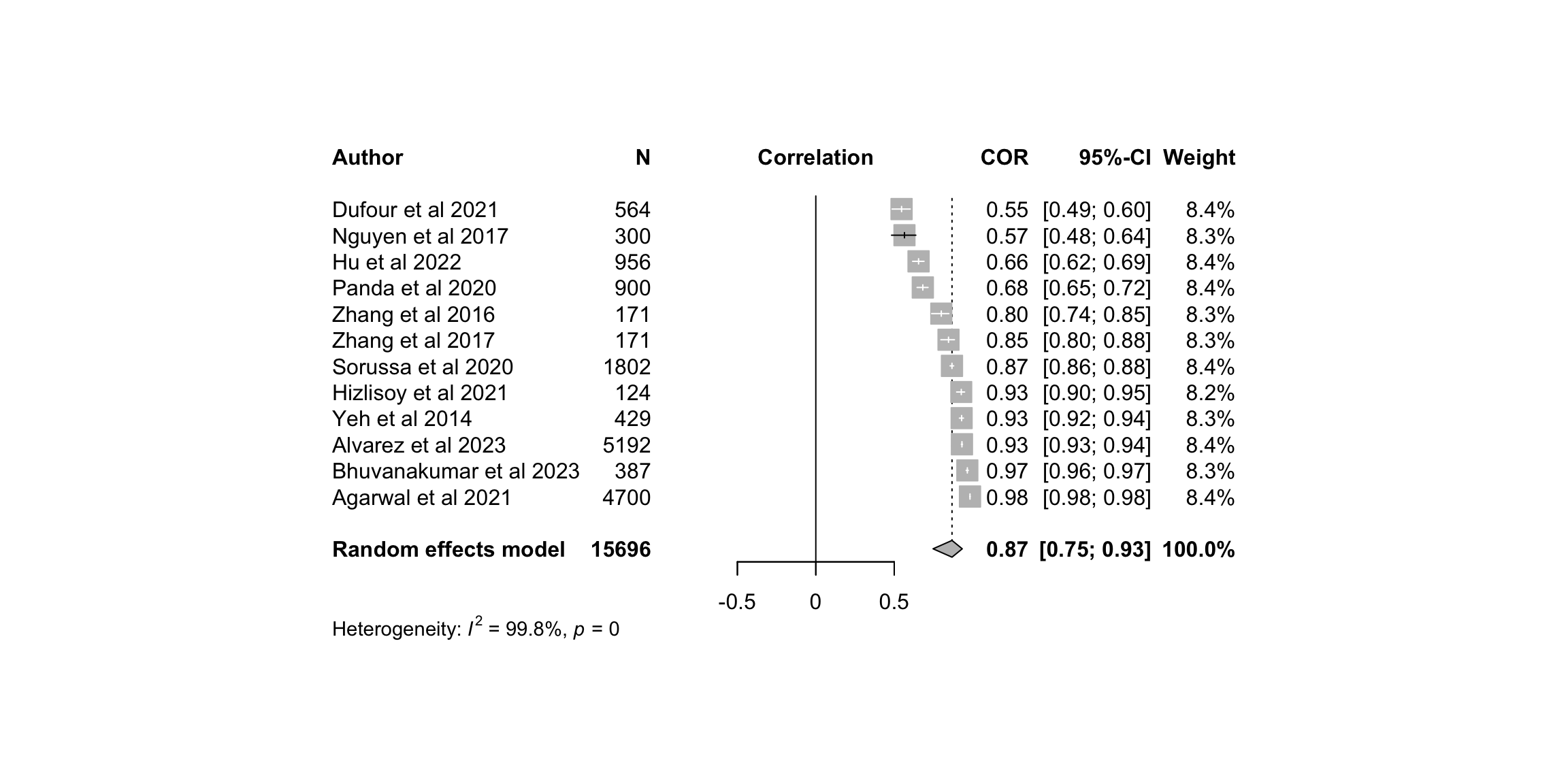
fig3b<-funnel(m.cor.c, common = FALSE, studlab=TRUE,backtransf=TRUE)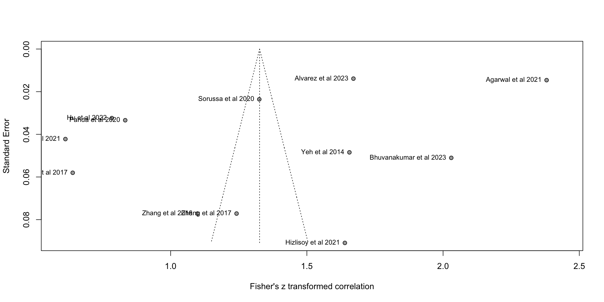
data<-tibble::tibble(mean=m.cor.c$cor,lower=FisherZInv(m.cor.c$lower),upper=FisherZInv(m.cor.c$upper),study=m.cor.c$studlab,n=m.cor.c$n,cor=round(m.cor.c$cor,2))
data<-dplyr::arrange(data,mean)

fp3 <- grid.grabExpr(print(data |>
                             forestplot(labeltext = c(study, n, cor),
                                        xlab = "Correlation",
                                        xticks = c(0, .25,.5,.75, 1),
                                        clip = c(0, 1))|>
                             fp_add_header(study = "Study",n = "N",cor = expression(italic(r))) |>
                             fp_append_row(mean  = m.cor.c$TE.common,
                                           lower = m.cor.c$lower.common,
                                           upper = m.cor.c$upper.common,
                                           study = "Summary",
                                           n = sum(m.cor.c$n),
                                           cor = round(m.cor.c$TE.common,2),
                                           is.summary = TRUE) |>
                             fp_set_style(box = "grey50",
                                          line = "grey20",
                                          summary = "black",
                                          txt_gp = fpTxtGp(label = list(gpar(cex = 0.80)),
                                                           ticks = gpar(cex = 0.80),
                                                           xlab  = gpar(cex = 0.80)))|>
                             fp_decorate_graph(grid = structure( m.cor.c$TE.common,gp = gpar(lty = 2, col = "grey30")))
)
)

source('../etc/custom_funnel_plot.R')
fp4 <- custom_funnel_plot(m.cor.c)

gridExtra::grid.arrange(fp3, fp4, ncol=2, widths=c(2,1),heights=c(2,1))
Warning: Removed 984 rows containing missing values or values outside the scale range
(`geom_line()`).
Removed 984 rows containing missing values or values outside the scale range
(`geom_line()`).Warning: Removed 1 row containing missing values or values outside the scale range
(`geom_hline()`).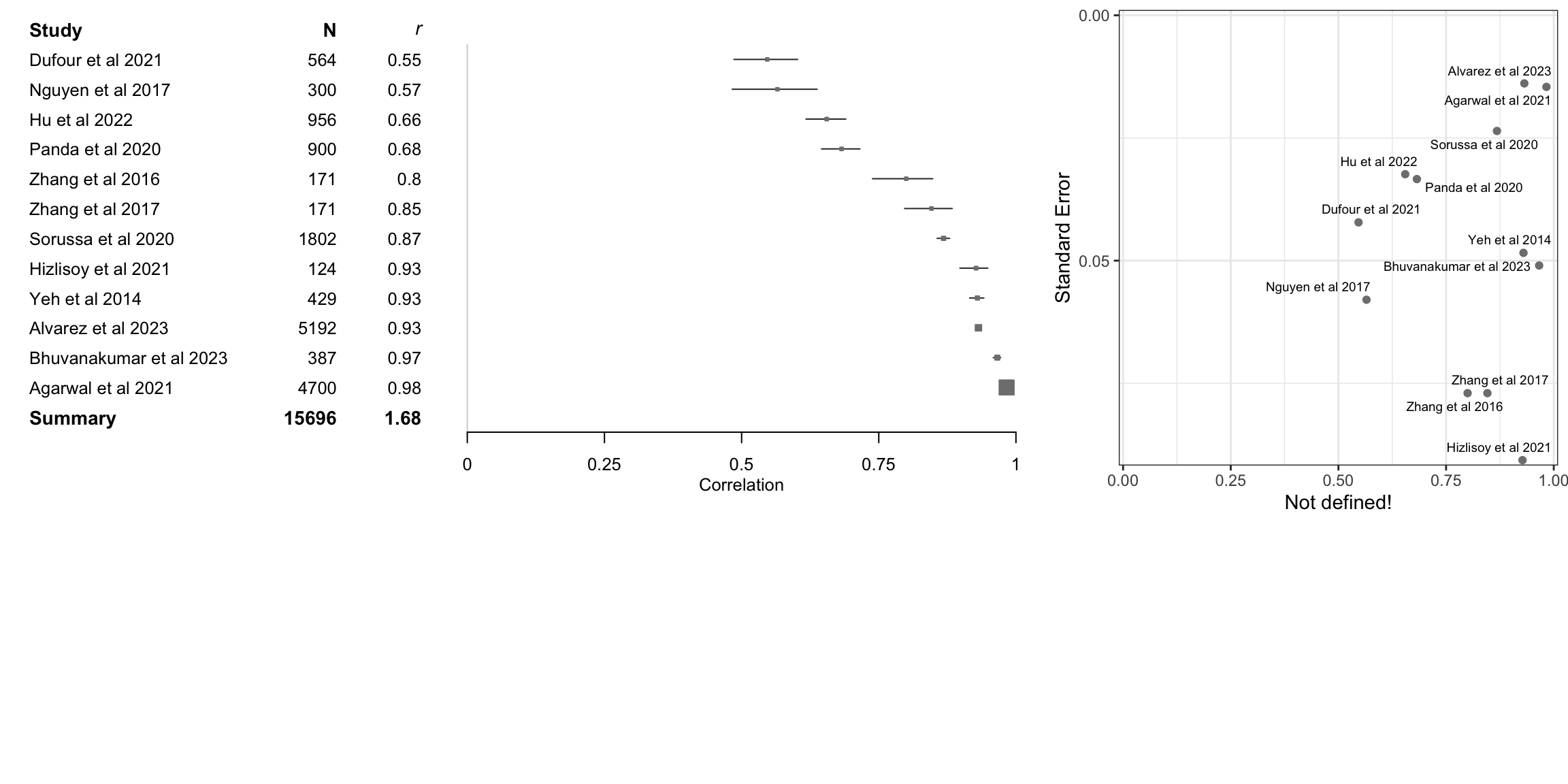
Exploring heterogeneity
# Method 1: Give us the Egger's test about beta coefficient from funnel
print(eggers.test(m.cor.c))
Eggers' test of the intercept
=============================
intercept 95% CI t p
-19.769 -39.29 - -0.24 -1.984 0.07531011
Eggers' test does not indicate the presence of funnel plot asymmetry. # Method 2: Find the impact to the results when removing those outside the 95CI
O <- find.outliers(m.cor.c) # 13 remaining out of 24
print(O)Identified outliers (random-effects model)
------------------------------------------
"Agarwal et al 2021", "Bhuvanakumar et al 2023", "Dufour et al 2021", "Hu et al 2022", "Nguyen et al 2017", "Panda et al 2020"
Results with outliers removed
-----------------------------
Review: MER: Classification: Summary
Number of studies: k = 6
Number of observations: o = 7889
COR 95%-CI t p-value
Random effects model 0.8941 [0.8282; 0.9356] 14.29 < 0.0001
Prediction interval [0.6506; 0.9709]
Quantifying heterogeneity (with 95%-CIs):
tau^2 = 0.0569 [0.0199; 0.3670]; tau = 0.2385 [0.1410; 0.6058]
I^2 = 97.7% [96.6%; 98.5%]; H = 6.63 [5.39; 8.15]
Test of heterogeneity:
Q d.f. p-value
219.67 5 < 0.0001
Details of meta-analysis methods:
- Inverse variance method
- Restricted maximum-likelihood estimator for tau^2
- Q-Profile method for confidence interval of tau^2 and tau
- Calculation of I^2 based on Q
- Hartung-Knapp adjustment for random effects model (df = 5)
- Prediction interval based on t-distribution (df = 5)
- Fisher's z transformation of correlations# Method 3: Leave-out-out analysis etc for individual influence (not useful here)
#infan <- InfluenceAnalysis(m.cor)
# Method 4: Focus on 10% of most precise studies (Stanley, Jarrel, Doucouliagos 2010)
thres<-quantile(m.cor.c$seTE,0.1)
ind<-m.cor.c$seTE<=as.numeric(thres)
m.cor10pct <- update(m.cor.c, subset = which(ind))
# Method 5: P curve analysis (Simonsohn, Simmons & Nelson, 2015)
pcurve(m.cor.c)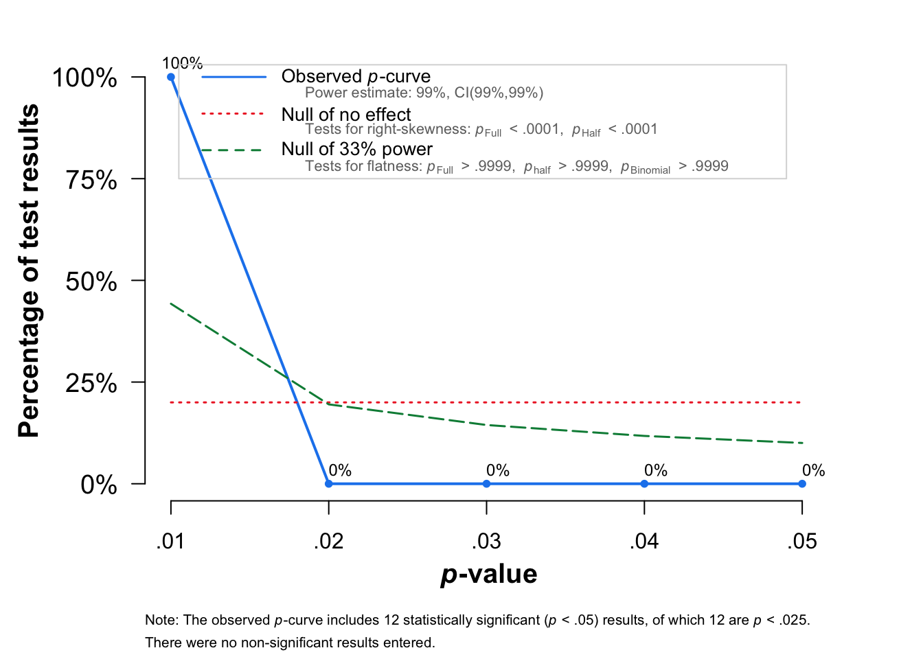
P-curve analysis
 -----------------------
- Total number of provided studies: k = 12
- Total number of p<0.05 studies included into the analysis: k = 12 (100%)
- Total number of studies with p<0.025: k = 12 (100%)

Results
 -----------------------
                    pBinomial   zFull pFull   zHalf pHalf
Right-skewness test         0 -26.866     0 -26.559     0
Flatness test               1  28.149     1  28.149     1
Note: p-values of 0 or 1 correspond to p<0.001 and p>0.999, respectively.
Power Estimate: 99% (99%-99%)

Evidential value
 -----------------------
- Evidential value present: yes
- Evidential value absent/inadequate: no
Re-run the analysis without outliers
Visualise (forest and funnel plots)
forest(m.cor.c.o,
       sortvar = TE,
       prediction = FALSE,
             print.tau2 = FALSE,
             leftlabs = c("Author", "N"),studlab = citekey)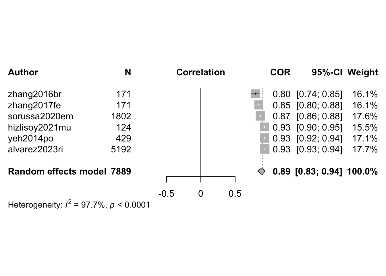
funnel(m.cor.c.o, common = FALSE, studlab=TRUE,backtransf=TRUE)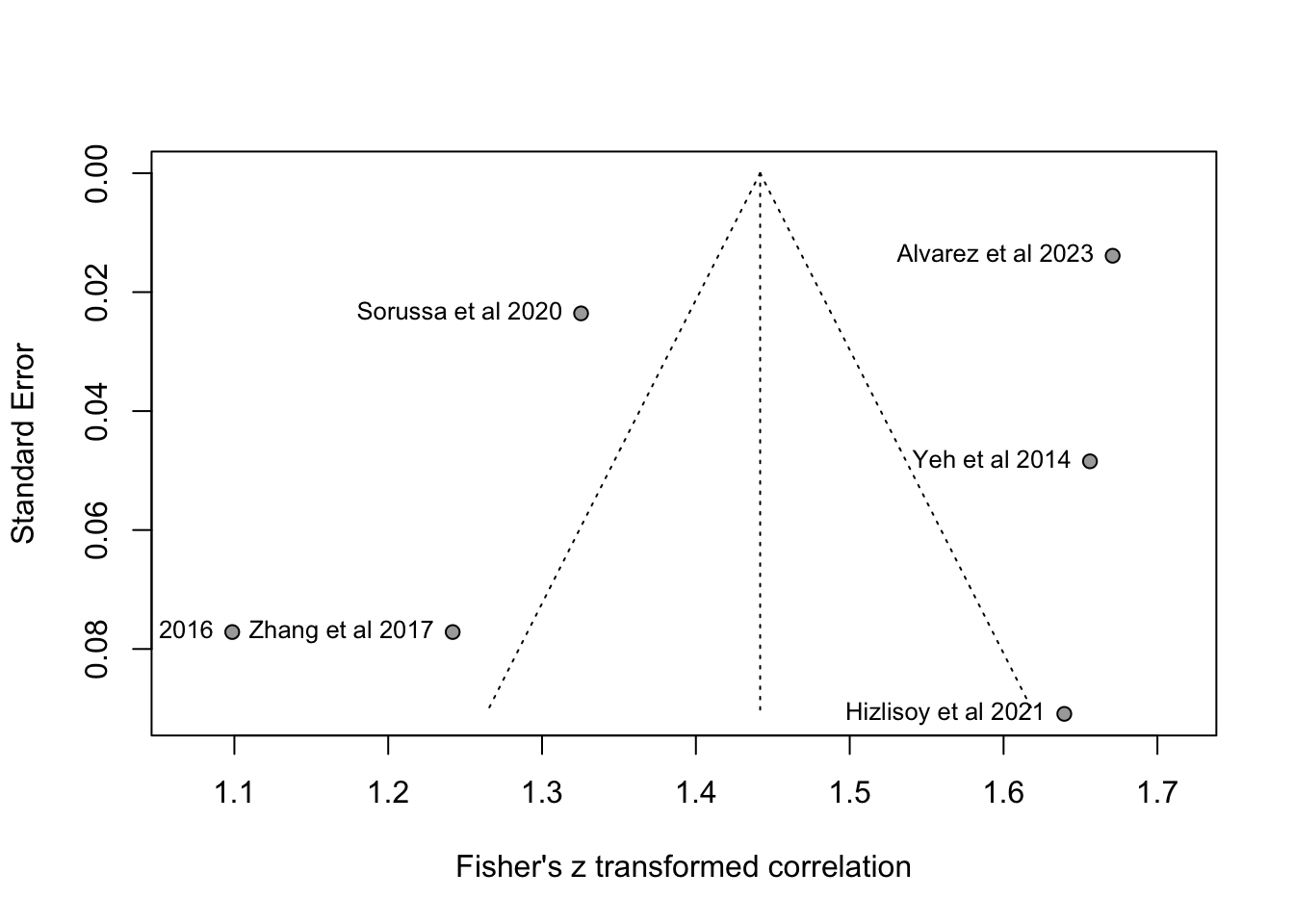
Subgroup analyses
By binary vs. multi-class classification
m.cor_classes <- update(
  m.cor.c,
  subgroup = classes)

print(m.cor_classes)
Review: MER: Classification: Summary
Number of studies: k = 12
Number of observations: o = 15696
COR 95%-CI t p-value
Random effects model 0.8684 [0.7475; 0.9336] 8.13 < 0.0001
Prediction interval [0.0341; 0.9894]
Quantifying heterogeneity (with 95%-CIs):
tau^2 = 0.3180 [0.1582; 0.9169]; tau = 0.5639 [0.3977; 0.9576]
I^2 = 99.8%; H = 21.39
Test of heterogeneity:
Q d.f. p-value
5031.22 11 0
Results for subgroups (random effects model):
k COR 95%-CI tau^2 tau Q I^2
classes = Multiclass 8 0.8729 [0.6804; 0.9527] 0.3783 0.6151 4069.76 99.8%
classes = Binary 4 0.8588 [0.4162; 0.9724] 0.2801 0.5293 426.79 99.3%
Test for subgroup differences (random effects model):
Q d.f. p-value
Between groups 0.03 1 0.8694
Details of meta-analysis methods:
- Inverse variance method
- Restricted maximum-likelihood estimator for tau^2
- Q-Profile method for confidence interval of tau^2 and tau
- Calculation of I^2 based on Q
- Hartung-Knapp adjustment for random effects model (df = 11)
- Prediction interval based on t-distribution (df = 11)
- Fisher's z transformation of correlationsforest(m.cor_classes,
sortvar = TE,
prediction = FALSE,
print.tau2 = FALSE,
leftlabs = c("Author", "N"),
studlab = citekey)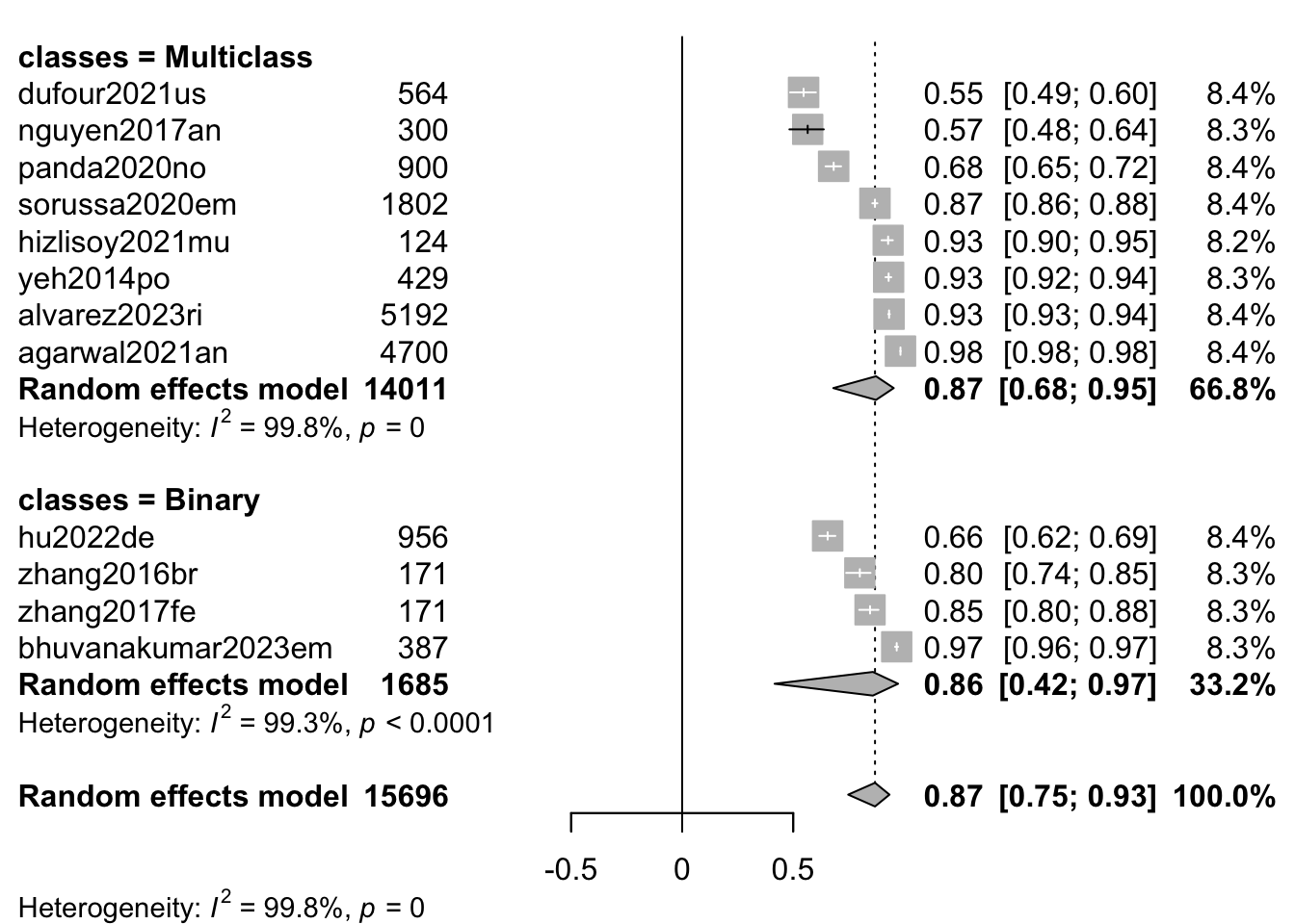
funnel(m.cor, common = FALSE, studlab=TRUE,backtransf=TRUE)
By journal type
m.cor_journal <- update(
  m.cor.c,
  subgroup = journal_type
)

print(m.cor_journal)
Review: MER: Classification: Summary
Number of studies: k = 12
Number of observations: o = 15696
COR 95%-CI t p-value
Random effects model 0.8684 [0.7475; 0.9336] 8.13 < 0.0001
Prediction interval [0.0341; 0.9894]
Quantifying heterogeneity (with 95%-CIs):
tau^2 = 0.3180 [0.1582; 0.9169]; tau = 0.5639 [0.3977; 0.9576]
I^2 = 99.8%; H = 21.39
Test of heterogeneity:
Q d.f. p-value
5031.22 11 0
Results for subgroups (random effects model):
k COR 95%-CI tau^2 tau Q
journal_type = Engineering 12 0.8684 [0.7475; 0.9336] 0.3180 0.5639 5031.22
I^2
journal_type = Engineering 99.8%
Test for subgroup differences (random effects model):
Q d.f. p-value
Between groups 0.00 0 --
Details of meta-analysis methods:
- Inverse variance method
- Restricted maximum-likelihood estimator for tau^2
- Q-Profile method for confidence interval of tau^2 and tau
- Calculation of I^2 based on Q
- Hartung-Knapp adjustment for random effects model (df = 11)
- Prediction interval based on t-distribution (df = 11)
- Fisher's z transformation of correlationsBy single vs. multi-genre
m.cor_subgroups <- update(
  m.cor.c,
  subgroup = stimulus_genre_mixed
)

print(m.cor_subgroups)
#forest(m.cor_subgroups,subgroup=TRUE)
By feature complexity
m.cor_complexity <- update(
  m.cor.c,
  subgroup = feature_n_complexity
)

print(m.cor_complexity)
Review: MER: Classification: Summary
Number of studies: k = 12
Number of observations: o = 15696
COR 95%-CI t p-value
Random effects model 0.8684 [0.7475; 0.9336] 8.13 < 0.0001
Prediction interval [0.0341; 0.9894]
Quantifying heterogeneity (with 95%-CIs):
tau^2 = 0.3180 [0.1582; 0.9169]; tau = 0.5639 [0.3977; 0.9576]
I^2 = 99.8%; H = 21.39
Test of heterogeneity:
Q d.f. p-value
5031.22 11 0
Results for subgroups (random effects model):
k COR 95%-CI
feature_n_complexity = Feature n > 30 & < 300 5 0.8458 [ 0.3613; 0.9707]
feature_n_complexity = Feature n < 30 4 0.9293 [ 0.8160; 0.9738]
feature_n_complexity = Feature n > 300 3 0.7754 [-0.2709; 0.9818]
tau^2 tau Q I^2
feature_n_complexity = Feature n > 30 & < 300 0.4822 0.6944 3839.01 99.9%
feature_n_complexity = Feature n < 30 0.0978 0.3127 79.97 96.2%
feature_n_complexity = Feature n > 300 0.2724 0.5219 88.46 97.7%
Test for subgroup differences (random effects model):
Q d.f. p-value
Between groups 3.91 2 0.1419
Details of meta-analysis methods:
- Inverse variance method
- Restricted maximum-likelihood estimator for tau^2
- Q-Profile method for confidence interval of tau^2 and tau
- Calculation of I^2 based on Q
- Hartung-Knapp adjustment for random effects model (df = 11)
- Prediction interval based on t-distribution (df = 11)
- Fisher's z transformation of correlationsBy model type
m.cor_subgroups <- update(
  m.cor.c,
  subgroup = model_class_id,
)

print(m.cor_subgroups)
#forest(m.cor_subgroups,subgroup=TRUE)
Custom funnel plot
To show the quality differences between core and eliminated studies (in progress).
tmpdata <- data.frame(SE = m.cor.c$seTE, Zr = m.cor.c$TE, studies=m.cor.c$studlab)

tmpdata$studyREF <- substr(tmpdata$studies,1,nchar(tmpdata$studies)-2)
tmpdata$studyREF <- str_replace_all(tmpdata$studyREF,'([0-9]+)',' et al \\1')
tmpdata$studyREF <- str_to_sentence(tmpdata$studyREF)
tmpdata$studyREF
[1] "Agarwal et al et al 20" "Alvarez et al et al 20"
[3] "Bhuvanakumar et al et al 20" "Dufour et al et al 20"
[5] "Hizlisoy et al et al 20" "Hu et al et al 20"
[7] "Nguyen et al et al 20" "Panda et al et al 20"
[9] "Sorussa et al et al 20" "Yeh et al et al 20"
[11] "Zhang et al et al 20" "Zhang et al et al 20" estimate = m.cor.c$TE.common
se = m.cor.c$seTE.common
se.seq=seq(0, max(m.cor.c$cor), 0.001)
ll95 = estimate-(1.96*se.seq)
ul95 = estimate+(1.96*se.seq)
ll99 = estimate-(3.29*se.seq)
ul99 = estimate+(3.29*se.seq)
meanll95 = estimate-(1.96*se)
meanul95 = estimate+(1.96*se)
dfCI = data.frame(ll95, ul95, ll99, ul99, se.seq, estimate, meanll95, meanul95)
fp = ggplot(NULL) +
geom_point(aes(x = SE, y = Zr), color='grey50',data=tmpdata) +
geom_text_repel(aes(x = SE, y = Zr, label=studyREF), data=tmpdata,size=2.5,max.overlaps = 40)+
xlab('Standard Error') + ylab('Fisher\'s z transformed correlation')+
geom_line(aes(x = se.seq, y = ll95), linetype = 'dotted', data = dfCI) +
geom_line(aes(x = se.seq, y = ul95), linetype = 'dotted', data = dfCI) +
geom_segment(aes(x = min(se.seq), y = meanll95, xend = max(se.seq), yend = meanll95), linetype='dotted', data=dfCI) +
geom_segment(aes(x = min(se.seq), y = meanul95, xend = max(se.seq), yend = meanul95), linetype='dotted', data=dfCI) +
# scale_x_reverse()+
scale_x_reverse(breaks=seq(0,0.2,0.05),limits=c(0.15,0),expand=c(0.00,0.00))+
# scale_y_continuous(breaks=seq(0.3,1.25,0.20),limits=c(0.3,1.23))+
coord_flip()+
theme_bw()
print(fp)Warning: Removed 833 rows containing missing values or values outside the scale range
(`geom_line()`).
Removed 833 rows containing missing values or values outside the scale range
(`geom_line()`).Warning: Removed 984 rows containing missing values or values outside the scale range
(`geom_segment()`).
Removed 984 rows containing missing values or values outside the scale range
(`geom_segment()`).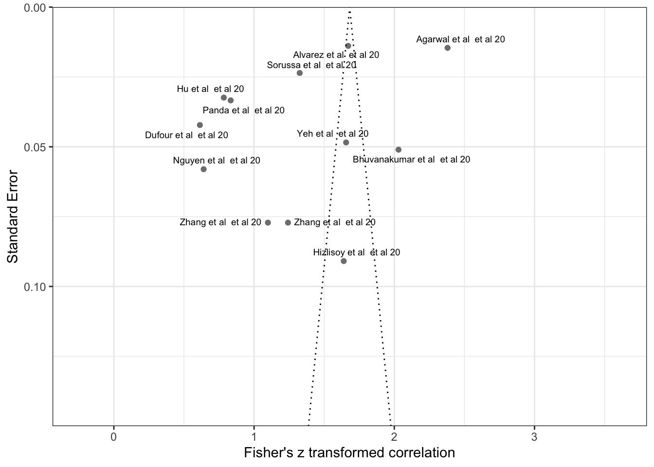
- Idea: visualise the distributions of the model successes within studies (done in preprocessing)